We now describe the celebrated Upper Confidence Bound (UCB) algorithm that overcomes all of the limitations of strategies based on exploration followed by commitment, including the need to know the horizon and sub-optimality gaps. The algorithm has many different forms, depending on the distributional assumptions on the noise.

Optimism in the face of uncertainty but on overdose: Not recommended!
The algorithm is based on the principle of optimism in the face of uncertainty, which is to choose your actions as if the environment (in this case bandit) is as nice as is plausibly possible. By this we mean that the unknown mean payoffs of each arm is as large as plausibly possible based on the data that has been observed (unfounded optimism will not work — see the illustration on the right!). The intuitive reason that this works is that when acting optimistically one of two things happens. Either the optimism was justified, in which case the learner is acting optimally, or the optimism was not justified. In the latter case the agent takes some action that they believed might give a large reward when in fact it does not. If this happens sufficiently often, then the learner will learn what is the true payoff of this action and not choose it in the future. The careful reader may notice that this explains why this rule will eventually get things right (it will be “consistent” in some sense), but the argument does not quite explain why an optimistic algorithm should actually be a good algorithm among all consistent ones. However, before getting to this, let us clarify what we mean by plausible.
Recall that if $X_1, X_2,\ldots, X_n$ are independent and $1$-subgaussian (which means that $\E[X_i] = 0$) and $\hat \mu = \sum_{t=1}^n X_t / n$, then
\begin{align*}
\Prob{\hat \mu \geq \epsilon} \leq \exp\left(-n\epsilon^2 / 2\right)\,.
\end{align*}
Equating the right-hand side with $\delta$ and solving for $\epsilon$ leads to
\begin{align}
\label{eq:simple-conc}
\Prob{\hat \mu \geq \sqrt{\frac{2}{n} \log\left(\frac{1}{\delta}\right)}} \leq \delta\,.
\end{align}
This analysis immediately suggests a definition of “as large as plausibly possible”. Using the notation of the previous post, we can say that when the learner is deciding what to do in round $t$ it has observed $T_i(t-1)$ samples from arm $i$ and observed rewards with an empirical mean of $\hat \mu_i(t-1)$ for it. Then a good candidate for the largest plausible estimate of the mean for arm $i$ is
\begin{align*}
\hat \mu_i(t-1) + \sqrt{\frac{2}{T_i(t-1)} \log\left(\frac{1}{\delta}\right)}\,.
\end{align*}
Then the algorithm chooses the action $i$ that maximizes the above quantity. If $\delta$ is chosen very small, then the algorithm will be more optimistic and if $\delta$ is large, then the optimism is less certain. We have to be very careful when comparing the above display to \eqref{eq:simple-conc} because in one the number of samples is the constant $n$ and in the other it is a random variable $T_i(t-1)$. Nevertheless, this is in some sense a technical issue (that needs to be taken care of properly, of course) and the intuition remains that $\delta$ is approximately an upper bound on the probability of the event that the above quantity is an underestimate of the true mean.
The value of $1-\delta$ is called the confidence level and different choices lead to different algorithms, each with their pros and cons, and sometimes different analysis. For now we will choose $1/\delta = f(t)= 1 + t \log^2(t)$, $t=1,2,\dots$. That is, $\delta$ is time-dependent, and is decreasing to zero slightly faster than $1/t$. Readers are not (yet) expected to understand this choice whose pros and cons we will discuss later. In summary, in round $t$ the UCB algorithm will choose arm $A_t$ given by
\begin{align}
A_t = \begin{cases}
\argmax_i \left(\hat \mu_i(t-1) + \sqrt{\frac{2 \log f(t)}{T_i(t-1)}}\right)\,, & \text{if } t > K\,; \\
t\,, & \text{otherwise}\,.
\end{cases}
\label{eq:ucb}
\end{align}
The reason for the cases is that the term inside the square root is undefined if $T_i(t-1) = 0$ (as it is when $t = 1$), so we will simply have the algorithm spend the first $K$ rounds choosing each arm once. The value inside the argmax is called the index of arm $i$. Generally speaking, an index algorithm chooses the arm in each round that maximizes some value (the index), which usually only depends on current time-step and the samples from that arm. In the case of UCB, the index is the sum of the empirical mean of rewards experienced and the so-called exploration bonus, also known as the confidence width.
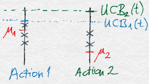
Illustration of UCB with 2 actions. The true means are shown in red ink. The observations are shown by crosses. Action 2 received fewer observations than Action 1. Hence, although its empirical mean is about the same as that of Action 1, Action 2 will be chosen in the next round.
Besides the slightly vague “optimism guarantees optimality or learning” intuition we gave before, it is worth exploring other intuitions for this choice of index. At a very basic level, we should explore arms more often if they are (a) promising (in that $\hat \mu_i(t-1)$ is large) or (b) not well explored ($T_i(t-1)$ is small). As one can plainly see from the definition, the UCB index above exhibits this behaviour. This explanation is unsatisfying because it does not explain why the form of the functions is just so.
An alternative explanation comes from thinking of what we expect from any reasonable algorithm. Suppose in some round we have played some arm (let’s say arm $1$) much more frequently than the others. If we did a good job designing our algorithm we would hope this is the optimal arm. Since we played it so much we can expect that $\hat \mu_1(t-1) \approx \mu_1$. To confirm the hypothesis that arm $1$ is indeed optimal the algorithm better be highly confident about that other arms are indeed worse. This leads very naturally to confidence intervals and the requirement that $T_i(t-1)$ for other arms $i\ne 1$ better be so large that
\begin{align}\label{eq:ucbconstraint}
\hat \mu_i(t-1) + \sqrt{\frac{2}{T_i(t-1)} \log\left(\frac{1}{\delta}\right)} \leq \mu_1\,,
\end{align}
because, at a confidence level of $1-\delta$ this guarantees that $\mu_i$ is smaller than $\mu_1$ and if the above inequality did not hold, the algorithm would not be justified in choosing arm $1$ much more often than arm $i$. Then, planning for $\eqref{eq:ucbconstraint}$ to hold makes it reasonable to follow the UCB rule as this will eventually guarantee that this inequality holds when arm $1$ is indeed optimal and arm $i$ is suboptimal. But how to choose $\delta$? If the confidence interval fails, by which we mean, if actually it turns out that arm $i$ is optimal and by unlucky chance it holds that
\begin{align*}
\hat \mu_i(t-1) + \sqrt{\frac{2}{T_i(t-1)} \log\left(\frac{1}{\delta}\right)} \leq \mu_i\,,
\end{align*}
then arm $i$ can be disregarded even though it is optimal. In this case the algorithm may pay linear regret (in $n$), so it better be the case that the failure occurs with about $1/n$ probability to fix the upper bound on the expected regret to be constant for the case when the confidence interval fails. Approximating $n \approx t$ leads then (after a few technicalities) to the choice of $f(t)$ in the definition of UCB given in \eqref{eq:ucb}. With this much introduction, we state the main result of this post:
Theorem (UCB Regret): The regret of UCB is bounded by
\begin{align} \label{eq:ucbbound}
R_n \leq \sum_{i:\Delta_i > 0} \inf_{\epsilon \in (0, \Delta_i)} \Delta_i\left(1 + \frac{5}{\epsilon^2} + \frac{2}{(\Delta_i – \epsilon)^2} \left( \log f(n) + \sqrt{\pi \log f(n)} + 1\right)\right)\,.
\end{align}
Furthermore,
\begin{align} \label{eq:asucbbound}
\displaystyle \limsup_{n\to\infty} R_n / \log(n) \leq \sum_{i:\Delta_i > 0} \frac{2}{\Delta_i}\,.
\end{align}
Note that in the first display, $\log f(n) \approx \log(n) + 2\log\log(n)$. We thus see that this bound scales logarithmically with the length of the horizon and is able to essentially reproduce the bound that we obtained for the unfeasible version of ETC with $K=2$ (when we tuned the exploration time based on the knowledge of $\Delta_2$). We shall discuss further properties of this bound later, but now let us present a simpler version of the above bound, avoiding all these epsilons and infimums that make for a confusing theorem statement. By choosing $\epsilon = \Delta_i/2$ inside the sum leads to the following corollary:
Corollary (UCB Simplified Regret): The regret of UCB is bounded by
\begin{align*}
R_n \leq \sum_{i:\Delta_i > 0} \left(\Delta_i + \frac{1}{\Delta_i}\left(8 \log f(n) + 8\sqrt{\pi \log f(n)} + 28\right)\right)\,.
\end{align*}
and in particular there exists some universal constant $C>0$ such that for all $n\ge 2$, $R_n \le \sum_{i:\Delta_i>0} \left(\Delta_i + \frac{C \log n}{\Delta_i}\right)$.
Note that taking the limit of the ratio of the bound above and $\log(n)$ does not result in the same rate as in the theorem, which is the main justification for introducing the epsilons in the first place. In fact, as we shall see the asymptotic bound on the regret given in \eqref{eq:asucbbound}, which is derived from~\eqref{eq:ucbbound} by choosing $\epsilon = \log^{-1/4}(n)$, is unimprovable in a strong sense.
The proof of the theorem relies on the basic regret decomposition identity that expresses the expected regret as the weighted sum of the expected number of times the suboptimal actions are chosen. So why will $\EE{T_i(n)}$ be small for a suboptimal action $i$? This is based on a couple of simple observations: First, (disregarding the initial period when all arms are chosen once) the suboptimal action $i$ can only be chosen if its UCB index is higher than that of an optimal arm. Now, this can only happen if the UCB index of action $i$ is “too high”, i.e., higher than $\mu^*-\epsilon>\mu_i$ or the UCB index of that optimal arm is “too low”, i.e., if it is below $\mu^*-\epsilon<\mu^*$. Since the UCB index of any arm is with reasonably high probability an upper bound on the arm’s mean, we don’t expect the index of any arm to be below its mean. Hence, the total number of times when the optimal arm’s index is “too low” (as defined above) is expected to be negligibly small. Furthermore, if the sub-optimal arm $i$ is played sufficiently often, then its exploration bonus becomes small and simultaneously the empirical estimate of its mean converges to the true value, making the expected total number of times when its index stays above $\mu^*-\epsilon$ small.
We start with a useful lemma that will help us quantify the last argument.
Lemma Let $X_1,X_2,\ldots$ be a sequence of independent $1$-subgaussian random variables, $\hat \mu_t = \sum_{s=1}^t X_s / t$, $\epsilon > 0$ and
\begin{align*}
\kappa = \sum_{t=1}^n \one{\hat \mu_t + \sqrt{\frac{2a}{t}} \geq \epsilon}\,.
\end{align*}
Then, $\displaystyle \E[\kappa] \leq 1 + \frac{2}{\epsilon^2} (a + \sqrt{\pi a} + 1)$.
Because the $X_i$ are $1$-subgaussian and independent we have $\E[\hat \mu_t] = 0$, so we cannot expect $\hat \mu_t + \sqrt{2a/t}$ to be smaller than $\epsilon$ until $t$ is at least $2a/\epsilon^2$. The lemma confirms that this is indeed of the right order as an estimate for $\EE{\kappa}$.
Proof
Let $u = 2a \epsilon^{-2}$. Then, by the concentration theorem for subgaussian variables,
\begin{align*}
\E[\kappa]
&\leq u + \sum_{t=\ceil{u}}^n \Prob{\hat \mu_t + \sqrt{\frac{2a}{t}} \geq \epsilon} \\
&\leq u + \sum_{t=\ceil{u}}^n \exp\left(-\frac{t\left(\epsilon – \sqrt{\frac{2a}{t}}\right)^2}{2}\right) \\
&\leq 1 + u + \int^\infty_u \exp\left(-\frac{t\left(\epsilon – \sqrt{\frac{2a}{t}}\right)^2}{2}\right) dt \\
&= 1 + \frac{2}{\epsilon^2}(a + \sqrt{\pi a} + 1)\,.
\end{align*}
QED
Before the proof of the UCB regret theorem we need a brief diversion back to the bandit model. We have defined $\hat \mu_i(t)$ as the empirical mean of the $i$th arm after the $t$th round, which served us well enough for the analysis of the explore-then-commit strategy where the actions were chosen following a deterministic rule. For UCB it is very useful also to have $\hat \mu_{i,s}$, the empirical average of the $i$th arm after $s$ observations from that arm, which occurs at a random time (or maybe not at all). To define $\hat \mu_{i,s}$ rigorously, we argue that without the loss of generality one may assume that the reward $X_t$ received in round $t$ comes from choosing the $T_i(t)$th element from the reward sequence $(Z_{i,s})_{1\le s \le n}$ associated with arm $i$, where $(Z_{i,s})_s$ is an i.i.d. sequence with $Z_{i,s}\sim P_i$. Formally,
\begin{align}\label{eq:rewardindepmodel}
X_t = Z_{A_t,T_{A_t}(t)}\,.
\end{align}
The advantage of introducing $(Z_{i,s})_s$ is that it allows a clean definition (without $Z_{i,s}$, how does one even define $\hat \mu_{i,s}$ if $T_i(n) \leq s$?). In particular, we let
\begin{align*}
\hat \mu_{i,s} &= \frac{1}{s} \sum_{u=1}^s Z_{i,u}\,.
\end{align*}
Note that $\hat \mu_{i,s} = \hat \mu_i(t)$ when $T_i(t)=s$ (formally: $\hat \mu_{i,T_i(t)} = \hat \mu_i(t)$).
Proof of Theorem
As in the analysis of the explore-then-commit strategy we start by writing the regret decomposition.
\begin{align*}
R_n = \sum_{i:\Delta_i > 0} \Delta_i \E[T_i(n)]\,.
\end{align*}
The rest of the proof revolves around bounding $\E[T_i(n)]$. Let $i$ be some sub-optimal arm (so that $\Delta_i > 0$). Following the suggested intuition we decompose $T_i(n)$ into two terms. The first measures the number of times the index of the optimal arm is less than $\mu_1 – \epsilon$. The second term measures the number of times that $A_t = i$ and its index is larger than $\mu_1 – \epsilon$.
\begin{align}
T_i(n)
&= \sum_{t=1}^n \one{A_t = i} \nonumber \\
&\leq \sum_{t=1}^n \one{\hat \mu_1(t-1) + \sqrt{\frac{2\log f(t)}{T_1(t-1)}} \leq \mu_1 – \epsilon} + \nonumber \\
&\qquad \sum_{t=1}^n \one{\hat \mu_i(t-1) + \sqrt{\frac{2 \log f(t)}{T_i(t-1)}} \geq \mu_1 – \epsilon \text{ and } A_t = i}\,. \label{eq:ucb1}
\end{align}
The proof of the first part of the theorem is completed by bounding the expectation of each of these two sums. Starting with the first, we again use the concentration guarantee.
\begin{align*}
\EE{\sum_{t=1}^n \one{\hat \mu_1(t-1) + \sqrt{\frac{2 \log f(t)}{T_1(t-1)}} \leq \mu_1 – \epsilon}}
&= \sum_{t=1}^n \Prob{\hat \mu_1(t-1) + \sqrt{\frac{2 \log f(t)}{T_1(t-1)}} \leq \mu_1 – \epsilon} \\
&\leq \sum_{t=1}^n \sum_{s=1}^n \Prob{\hat \mu_{1,s} + \sqrt{\frac{2 \log f(t)}{s}} \leq \mu_1 – \epsilon} \\
&\leq \sum_{t=1}^n \sum_{s=1}^n \exp\left(-\frac{s\left(\sqrt{\frac{2 \log f(t)}{s}} + \epsilon\right)^2}{2}\right) \\
&\leq \sum_{t=1}^n \frac{1}{f(t)} \sum_{s=1}^n \exp\left(-\frac{s\epsilon^2}{2}\right) \\
&\leq \frac{5}{\epsilon^2}\,.
\end{align*}
The first inequality follows from the union bound over all possible values of $T_1(t-1)$. This is an important point. The concentration guarantee cannot be applied directly because $T_1(t-1)$ is a random variable and not a constant. The last inequality is an algebraic exercise. The function $f(t)$ was chosen precisely so this bound would hold. If $f(t) = t$ instead, then the sum would diverge. Since $f(n)$ appears in the numerator below we would like $f$ to be large enough that its reciprocal is summable and otherwise as small as possible. For the second term in \eqref{eq:ucb1} we use the previous lemma.
\begin{align*}
&\EE{\sum_{t=1}^n \one{\hat \mu_i(t-1) + \sqrt{\frac{2 \log f(t)}{T_i(t-1)}} \geq \mu_1 – \epsilon \text{ and } A_t = i}} \\
&\qquad\leq \EE{\sum_{t=1}^n \one{\hat \mu_i(t-1) + \sqrt{\frac{2 \log f(n)}{T_i(t-1)}} \geq \mu_1 – \epsilon \text{ and } A_t = i}} \\
&\qquad\leq \EE{\sum_{s=1}^n \one{\hat \mu_{i,s} + \sqrt{\frac{2 \log f(n)}{s}} \geq \mu_1 – \epsilon}} \\
&\qquad= \EE{\sum_{s=1}^n \one{\hat \mu_{i,s} – \mu_i + \sqrt{\frac{2 \log f(n)}{s}} \geq \Delta_i – \epsilon}} \\
&\qquad\leq 1 + \frac{2}{(\Delta_i – \epsilon)^2} \left(\log f(n) + \sqrt{\pi \log f(n)} + 1\right)\,.
\end{align*}
The first part of the theorem follows by substituting the results of the previous two displays into \eqref{eq:ucb1}. The second part follows by choosing $\epsilon = \log^{-1/4}(n)$ and taking the limit as $n$ tends to infinity.
QED
Next week we will see that UCB is close to optimal in several ways. As with the explore-then-commit strategy, the bound given in the previous theorem is not meaningful when the gaps $\Delta_i$ are small. Like that algorithm it is possible to prove a distribution-free bound for UCB by treating the arms $i$ with small $\Delta_i$ differently. Fix $\Delta>0$ to be chosen later. Then, from the proof of the bound on the regret of UCB we can derive that $\EE{T_i(n)} \le \frac{C \log(n)}{\Delta_i^2}$ holds for all $n\ge 2$ with some universal constant $C>0$. Hence, the regret can be bounded without dependence on the sub-optimality gaps by
\begin{align*}
R_n
&= \sum_{i:\Delta_i > 0} \Delta_i \E[T_i(n)]
= \sum_{i:\Delta_i < \Delta} \Delta_i \E[T_i(n)] + \sum_{i:\Delta_i \geq \Delta} \Delta_i \E[T_i(n)] \\
&< n \Delta + \sum_{i:\Delta_i \geq \Delta} \Delta_i \E[T_i(n)]
\leq n \Delta + \sum_{i:\Delta_i \geq \Delta} \frac{C \log n}{\Delta_i} \\
&\leq n \Delta + K\frac{C \log n}{\Delta}
= \sqrt{C K n \log(n)}\,,
\end{align*}
where in the last step we chose $\Delta = \sqrt{K C \log(n) / n}$, which optimizes the upper bound.
There are many directions to improve or generalize this result. For example, if more is known about the noise model besides that it is subgaussian, then this can often be exploited to improve the regret. The main example is the Bernoulli case, where one should make use of the fact that the variance is small when the mean is close to zero or one. Another direction is improving the worst-case regret to match the lower bound of $\Omega(\sqrt{Kn})$ that we will see next week. This requires a modification of the confidence level and a more complicated analysis.
Notes
Note 1: Here we argue that there is no loss in generality in assuming that the rewards experienced satisfy $\eqref{eq:rewardindepmodel}$. Indeed, let $T’ = (A’_1,X’_1,\dots,A’_n,X’_n)$ be any sequence of random variables satisfying that $A_t’ = f_t(A’_1,X’_1,\dots,A’_{t-1},X’_{t-1})$ and that for any $U\subset \R$ open interval
\begin{align*}
\Prob{X_t’\in U\,|\,A’_1,X’_1,\dots,A’_{t-1},X’_{t-1},A’_t} = P_{A’_t}(U)\,,
\end{align*}
where $1\le t\le n$. Then, choosing $(Z_{i,s})_s$ as described in the paragraph before $\eqref{eq:rewardindepmodel}$, we let $T=(A_1,X_1,\dots,A_n,X_n)$ be such that $A_t = f_t(A_1,X_1,\dots,A_{t-1},X_{t-1})$ and $X_t$ be so that it satisfies $\eqref{eq:rewardindepmodel}$. It is not hard to see then that the distributions of $T$ and $T’$ agree. Hence, there is indeed no loss of generality by assuming that the rewards are indeed generated by $\eqref{eq:rewardindepmodel}$.
Note 2: The view that $n$ rewards are generated ahead of time for each arm and the algorithm consumes these rewards as it chooses an action was helpful in the proof as it reduced the argument to the study of averages of independent random variables. The analysis could also have been done directly without relying on the “virtual” rewards $(Z_{i,s})_s$ with the help of martingales, which we will meet later.
A third model of how $X_t$ is generated could have been that $X_t = Z_{A_t,t}$. We will meet this “skipping model” later when studying adversarial bandits. For the stochastic bandit models we study here, all these models coincide (they are indistinguishable in the sense described in the first note above).
Note 3: So is the optimism principle universal? Does it always give good algorithms, even in more complicated settings? Unfortunately, the answer is no. The optimism principle leads to reasonable algorithms when using an action gives feedback that informs the learner about how much the action is worth. If this is not true (i.e., in models where you have to choose action $B$ to learn about the rewards of action $A$, and choosing action $A$ would not give you information about the reward of action $A$), the principle fails! (Why?) Furthermore, even if all actions give information about their own value, the optimistic principle may give rise to algorithms whose regret is overly large compared to what could be achieved with more clever algorithms. Thus, in a way, finite-armed stochastic bandits is a perfect fit for optimistic algorithms. While the more complex feedback models may not make much sense at the moment, we will talk about them later.
References
The idea of using upper confidence bounds appeared in ’85 in the landmark paper of Lai and Robbins. In this paper they introduced a strategy which plays the leader of the “often sampled” actions except that for any action $j$ in every $K$th round the strategy is checking whether the UCB index of arm $j$ is higher than the estimated reward of the leader. They proved that this strategy, when appropriately tuned, is asymptotically unimprovable the same way UCB as we defined it is asymptotically unimprovable (we still owe the definition of this and a proof, which will come soon). The cleaner UCB idea must have been ready to be found in ’95 because Agrawal and Katehakis & Robbins discovered this idea independently in that year. Auer et al. later modified the strategy slightly and proved a finite-time analysis.
- Tzu L. Lai and Herbert Robbins. Asymptotically efficient adaptive allocation rules, 1985
- Rajeev Agrawal. Sample mean based index policies with $O(\log n)$ regret for the multi-armed bandit problem, 1995
- Michael N Katehakis and Herbert Robbins. Sequential choice from several populations, 1995
- Peter Auer, Nicolo Cesa-Bianchi, and Paul Fischer. Finite-time analysis of the multiarmed bandit problem, 2002

Sorry that I just can’t understand
why at a confidence level of 1−δ this guarantees that μi is smaller than μ1 and if the above inequality did not hold (after inequality (3))
The statement is slightly informal, but roughly $\hat \mu_i(t-1)$ is an empirical estimate of $\mu_i$ based on $T_i(t-1)$ samples. Since we assumed that the rewards are $1$-subgaussian we know that for $T_i(t-1) = u$ that $\Prob{\hat \mu_i + \sqrt{\frac{2}{u} \log\left(\frac{1}{\delta}\right)} \leq \mu_i} \leq \delta$. The informality comes from the fact that $T_i(t-1)$ is usually also a random variable, which makes the analysis a little trickier, but does not change much the intuition.
Note that we treat the concentration of subgaussian random variables in a previous post (https://banditalgs.com/2016/09/14/first-steps-explore-then-commit/)
Hi! Thanks for this amazing series of blogs.
I have a small question. I think it might be better to say that the value of 1-δ is called the confidence level (instead of saying δ is the confidence level). δ is sort of like the upper bound on the probability of error that we allow. Also, using 1-δ will possibly make it more consistent with confidence interval terminology used in statistics. Please correct me if I am wrong. Thanks! 🙂
You are right! I’ll fix this:) Thanks for the comment!
Hey Tor, do you mind expanding on inequality (7)? I sort of understand that the first and second terms in the inequality represent the events that the UCB index for the optimal arm is “too low” and that the UCB index for the sub-optimal arm is “too high”, respectively. However, I’m confused as to how either of these events imply that the UCB index for the sub-optimal arm is less than the UCB index for the optimal arm in a given round.
Hi,
I’ll dub as Tor. The implication is easiest to see by inverting things. We want to see that $A_t=i$ implies that $\UCB_i$ is high, or $\UCB_1$ is low. Well, if $\UCB_i$ was low and $\UCB_1$ was high, then arm $1$ would have been preferred to arm $i$, so it must be that if arm $i$ is selected then either $\UCB_i$ is high, or $\UCB_1$ is low. Does this make sense?
Cheers,
Csaba
PS: Sorry for the slow reply.
I am confused too about this inequality
In the first case ($UCB_1$ is low) the left hand side of the inequality is the index of arm 1, right? Shall we not use $T_1(t-1)$ in the denominator of the square root?
And why we compare the indices to $\mu_1 – \epsilon$? Why not simply $\mu_1?
Another good point. With $\epsilon=0$, what we would need to bound is the probability of the index of the optimal arm smaller than the optimal mean. The way the index is defined, if the optimal arm is pulled a fixed, say, $s$ number of times, this probability happens to be constant. This is too large; it would render the bound vacuous. I hope this helps. And sorry for the slow response; somehow I did not get a notification of the comment, or I just missed it.
Hmm, I have not caught this before. True. We should have had $T_1(t-1)$ in the denominator. I have corrected this now, thanks!
Hi Csaba, above you mentioned “The way the index is defined, if the optimal arm is pulled a fixed, say, s number of times, this probability happens to be constant.”
I am not really seeing how this is happening and how that would make it ‘too large’. Could you please explain this?
Hi, in the UCB Simplified Regret, does the universal constant C rely on suboptimality gaps? I suspect that if the suboptimality gaps are not bounded, we cannot find such a constant C.
Also, in the UCB regret (3), should the last constant be ‘1’, but not ‘3’?
Thank you!
Hi Xiang. You’re right on all counts. See the updated theorem for the (hopefully) correct statement of this kind of result.
Thanks for pointing out the bugs!
Tor
Great thanks for the quick response!
However, after the correction, there still exists a flaw in the final distribution-free bound for UCB. This bound also requires the suboptimality gaps be bounded, right?
Hi Xiang! Sorry for the slow response. Where is the bug? The universal constant just relies on bounding constant + $\log \log n$ by $C \log n$, it seems to me.
Hi, professor, when reasoning arm 1 is optimal and not the arm j (j \neq 1), we say that we have a 1-\delta level of confidence. But, should we also say arm 1 is optimal compared to all the other K-1 arms, so the confidence level would be (1-\delta)^{K-1}?
Where is this? The trick we use is that we bound the *expected* number of pulls of suboptimal arms. Hence, each suboptimal arm is compared to the optimal arm, one by one, separately, avoiding the need to argue about multiple suboptimal arms at the same time. I hope this clarifies things.
Hey!
It would be a big help for me if you could explain where the infimum condition in the equation for the UCB regret (Eq. (4)) comes from. It is comprehensible in the sense that one wants to keep the upper bound as small as possible, but why is the range of epsilon chosen like this?
By the way, thanks for creating this blog – I think this is a really nice medium to get into this topic!
Greetings,
You define 1/δ=f(t)=1+t*log²(t).
Most authors seem to define 1/δ=f(t)=t (see for example (1) in https://agrawal.wikischolars.columbia.edu/file/view/Lecture+3+part+1.pdf)
You can see that 1/δ in your (3) was replaced by t in his (1).
You do say “If f(t)=t instead, then the sum would diverge.” I am confused because everywhere I say UCB explained they use 1/δ=t…
I am implementing an UCB-based solution for a problem I have… Is there maybe a list of pros-and-cons of several f(t) functions? I could not find any, and I have tried to iterate the literature as much as I could…
Sorry if I am not making sense. I am a bandit newbie. 🙂
Hi Ricardo
The choice of f(t) is very delicate and one has to be careful about comparisons when the underlying variance is different. When the noise is Gaussian with variance V you generally want the confidence interval to look like
sqrt(2V / T_k log f(t))
where f(t) = t + O(log^p(t)) for as small p as your analysis will allow. Actually for the Gaussian case you may use f(t) = t, but even for subgaussian we do not know if this works. Roughly speaking things are easy if sum_t 1/f(t) converges. Now in Shipra’s notes the rewards are bounded in [0,1]. Of course they cannot be Gaussian, but the maximum variance (or subgaussian constant) of [0,1] bounded rewards is 1/4. If we substitute this into the formula above you have a confidence interval of
sqrt(2(1/4) / T_k log f(t)) = sqrt(1/(2T_k) log f(t))
Choosing f(t) = t^2 yields the choice in those notes and this is definitely summable. In general, if what you care about is expected regret, then you want f(t) to be “as small as possible”, but you will pay a price for this in terms of the variance of the regret, so take care. Finally, there are lots of more sophisticated choices. For example the arm-dependent confidence interval
sqrt(2V/T_k log(t/T_k)) will give you a big boost. I recently wrote a big literature review on all these choices. Feel free to email me if you want a copy.
Best,
Tor
I am suddenly a bit confused by the analysis for bounding the second term in eq (7). Why is the second inequality true. I understand that removing the intersection with $A_t = i$ gives an upper bound. But how do we deal with the change to $\hat{\mu}_{T_i(t-1)}$ to $\hat{\mu}_{i,s}$? Thanks for the nice write-up.
In the analysis after Eq. (7), why sum on s? Instead, you could write
… \le sum_{t=1}^n exp(-T_1(t-1)(epsilon + sqrt(2 lot f(t)/T_1(t-1)))^2)
\le sum_{t=1}^n exp(-T_1 esilon^2)/f(t)
\le sum_{t=1}^n 1/f(t)
This would be a stronger bound, although ultimately it wouldn’t change the scaling of regret with n. But am I missing something?
P.S. I love your blog!
The problem is that T_1(t-1) is a random variable, but we only proved the concentration guarantees hold for a fixed sample size. Actually the bounds do not hold more generally without slightly increasing the logarithmic term, which you can prove using the law of the iterated logarithm.
A little more directly, it’s always worth checking types. A (unconditional) probability should be a number so I better never write
P(predicate(X, Y)) <= f(X, Y)
because the left-hand side is a number and the right-hand side is a random quantity!
And thanks for the kind work. We hope you like the book even more!
I’ll admit — I didn’t totally understand that. Probably because I’m basically a physicist, so I’m sloppy when it comes to probabilities. 😉 But let me attempt to be more rigorous. Dropping the dependence on t-1, and using d1 as shorthand for \hat{\mu}_1(t-1) – \mu_1, we have
sum_t P(d1 + sqrt(2 log f(t)/T1) < -epsilon)
\le sum_t P(d1 + sqrt(2 log f(t)/T1) < 0)
= sum_t sum_T1 P(d1 + sqrt(2 log f(t)/T1) < 0|T1) P(T1)
\le sum_t (1/f(t)) sum_T1 P(T1)
= sum_t 1/f(t)
Is that any more correct?
Now the problem appears in the second inequality. When you condition on the number of samples T1 you change the underlying measure of the samples observed. Under this measure they are not independent so again the concentration bound cannot be applied. This is a bit counter intuitive, but hopefully the following example sheds some light on the issue.
Consider the case where the rewards are {0,1} valued and we are using a silly algorithm that plays arm 1 until it observes a zero and then plays other arms. When you condition on having played arm 1 some number of times (say, 100 times), then the empirical mean can only be 1 or 99/100 by the definition of the algorithm. But maybe the true mean is 1/2, which is not close at all to 1 or 99/100.
Of course the probability that this occurs is very small (because you are unlikely to ever observe 99 heads in a row. And this silly algorithm is not UCB. The point is just that by conditioning on the sample counts in problems involving sequential design is a risky business. Hence the naive union bound.
Thanks. That is indeed subtle.
Hi, thanks for posting theses. I have a small question about the sub-gaussian assumption(which leads to equation 1), do they have to have zero means? Or the equation should actually consider it’s mean and have a confidence band of the difference between empirical mean and the latent mean?
The usual definition is that X is 1-subgaussian if E[exp(lambda X)] <= exp(lambda^2/2) for all lambda. This definition implies that X has zero mean (proving this is a good exercise). In this post we are assuming that Z_{i,s} - mu_i is 1-subgaussian for all i and s.
I see, thank you for replying. Before, I thought the reward is assumed as a zero-mean subgaussian.
Now I’m confused about the union bound (going from the first to the second line in the equation after Eq. 7). Written in its most general form (suppressing the sum on n), it looks like
P(\hat{mu}(t-1) – mu_1 < g(n,T(t-1))) \le sum_s P(\hat{mu}(s) < g(n,s))
Presumably this should hold for arbitrary g(n,s). But I've been trying to convince myself of that for days, with no luck. Is there an easy way to see (or prove) it?
Thanks,
P
Hi
Let A_s be the event {T(t-1) = s and ^mu_s – mu <= g(s)}. Then the event F = {^mu_{T(t-1)} - mu <= g(T(t-1))} is a subset of the union of A_1,...,A_n since T(t-1) must be between 1 and n. Then the union bound says that Prob(F) <= Prob(union A_t) <= sum_t Prob(A_t)
That’s kind of what I thought. But then I started worrying: For the event F, ^mu_{T(t-1)} and T(t-1) are not independent, whereas for the event A_s, ^mu_s and s are independent. (OK, not quite independent, since s determines the variance of ^mu_s, but more independent than for F.)
I’m not sure what you’re getting at here. The independence of quantities that define F is not being used here. The union bound holds regardless of any independence.
The core is that F is indeed a subset of the union of all A_s and so the probability of F is less than the probability of the union. The second important part is that concentration analysis can bound the probability of A_s.
By the way, a slightly more straightforward analysis of a simpler algorithm is given in Chapter 7 of the book.
Let’s take a specific example, based on your example from an earlier thread:
x_i \in {0,1}; for definiteness let’s say P(x_i=1) = 1/2, so mu_i = 1/2.
strategy: choose arm i until x_i=1; then stop. under this strategy, if T_i = 3 then ^mu_i = 1/3.
let g(s) = 1/2 if s=3 and -1 if s \ne 3.
with this setup,
P(^mu(T_i=3) – mu_i < g(3)) = 1,
whereas
sum_s P(^mu_{i,s} – mu_i < g(s)) = P(^mu_{i,3} – mu_i < 1/2) < 1.
Thus, P(^mu(T_i=3) – mu_i < g(3)) is not less than sum_s P(^mu_{i,s} – mu_i < g(s)).
I'm guessing I have a serious misconception, but I can't figure out where.
Thanks,
Peter
P.S. The first time I left a comment, it took me forever to get past the robot with the missing eye, because its right eye is missing, and it asks to add the left eye. Is that part of the test? 😉
Hi
Probably the misconception is coming from your definition of P(^mu(T_i=3) – mu_i < g(3)). My interpretation of your argument is that this is meant to be a conditional probability. These are very difficult to handle in sequential settings and we avoid them. Our argument comes from the following view. To each arm associate a big stack of rewards, which are sampled independently at the beginning of the game and not observed. Each time the learner chooses an action, it gets the top reward on the stack corresponding to that arm. Then ^mu_{1,s} is the mean of the first s rewards in the stack corresponding to arm 1. Since these really are independent we can apply our concentration bound to show that with high probability ^mu_{1,s} + sqrt(2/s log f(t)) is never much smaller than mu_1 - epsilon for any s. Now the event F that ^mu_1(t-1) + sqrt(2/T_1(t-1) log f(t)) < mu_1 - epsilon is definitely a subset of the union of F_s with s in [n] where F_s is the event that ^mu_{1,s} + sqrt(2/s log f(t)) < mu_1 - epsilon. This is true because T_1(t-1) must be in [n] = {1,2,...,n}. Hence Prob(^mu_1(t-1) + sqrt(2/T_1(t-1) log f(t)) < mu_1 - epsilon) <= sum_{s=1}^n Prob(^mu_{1,s} + sqrt(2/s log f(t)) < mu_1 - epsilon)) Notice that in the left-hand side probability there is no conditioning. By the way, in the pdf book we have two versions of UCB, the first of which has slightly worse bounds than what we present here, but an easier proof (see Chapters 7 and 8).
I don’t really understand your argument, in the sense that it implies (to me) that P(^mu_i(t-1) – mu_i < g(T_i(t-1)) = P(^mu_{i,s} – mu_i < g(s)) and we know that's wrong.
But you are right that I'm interpreting the above probability as a conditional. If I instead thought of it as P((^mu_i(t-1) – mu_i < g(T_i(t-1)) & (T_i(t-1) was reached)), it makes much more sense. Under this interpretation, if I take the strategy of stopping when x_i=1, then (using my previous example) when T_i(t-1)=3:
P(^mu_i(t-1) – mu_i < g(3)) = P(observing 0, 0, 1 from arm i).
And in general, P(^mu_i(t-1) – mu_i < g(T_i(t-1)) is the probability of observing a particular set of data. Given that, the union bound makes perfect sense.
Is that a reasonably way of thinking about this?
I know you keep mentioning a simpler bound with an easier proof, but it's driving me nuts that I don't understand this one.
Thanks,
Peter
I think you’re on the right track. So indeed none of the probabilities in this post are conditional. $\Prob{A}$ is the probability that $A$ happens and in this case $A$ is the event that $\hat \mu_1(t-1) + \sqrt{2/T_1(t-1) \log f(t)} \le \mu_1 – \epsilon$.
Now we can write this event as a union of other events:
$A = \cup_s A_s$ where $A_s$ is the event that $\hat \mu_1(t-1) + \sqrt{2/T_1(t-1) \log f(t)} \le \mu_1 – \epsilon \text{ and } T_1(t-1) = s$.
On the event $A_s$ we have $T_1(t-1) = s$, so $A_s$ can also be written as the event that $\hat \mu_{1,s} + \sqrt{2/s \log f(t)} \le \mu_1 – \epsilon \text{ and } T_1(t-1) = s$. Now this is a subset of the event $B_s$ defined to occur when $\hat \mu_{1,s} + \sqrt{2/s \log f(t)} \le \mu_1 – \epsilon$ (clearly if $A_s$ happens, then $B_s$ also happens). So now we have $\Prob{A} = \Prob{\cup_s A_s} \le \sum_s \Prob{A_s} \le \sum_s \Prob{B_s}$.
First inequality is the union bound. Second inequality because $B_s$ is a subset of $A_s$. The price we pay for the fact that $T_1(t-1)$ is a random quantity is that we must sum over all its possible values when applying our concentration inequality.
Hi Csaba, above you mentioned “The way the index is defined, if the optimal arm is pulled a fixed, say, s number of times, this probability happens to be constant.”
I am not really seeing how this is happening and how that would make it ‘too large’. Could you please explain this?
Simply, plugging in $\epsilon=0$, we have $\Prob{\hat \mu_{1,s} + \sqrt{\frac{2 \log f(t)}{s}} \leq \mu_1}\le \exp\left(-\frac{s\left(\sqrt{\frac{2 \log f(t)}{s}} \right)^2}{2}\right)=\frac{1}{f(t)}$, which is too large for our purposes. I hope this makes sense.
I am wondering if we can also utilize the upper confidence bound for making life decisions?
Usually, the same life decision could not be made twice. That is, even if we are able to reduce uncertainty by making a specific choice, we would never be able to choose among the same alternative choices again. Is UCB still applicable in such situations?
UCB is not applicable in this case, for exactly the reason you point out. Life is a reinforcement learning problem, and a very difficult one.
Nevertheless, ideas based on optimism can work in reinforcement learning with some modification and assumptions. Somehow you need to construct confidence sets about what the world is like and then act as if the world is as nice as plausibly possible. You’ll have to make assumptions to do this.
Another big caveat. Optimism works well in bandits because you can never suffer too much regret with one wrong decision. This is obviously not true more generally. So caution is advised!
Tali Sharot’s book “Optimism Bias” is a nice exploration of optimistic behavior in humans, which maybe would interest you.