Continuing the previous post, here we give a construction for confidence bounds based on ellipsoidal confidence sets. We also put things together and show bound on the regret of the UCB strategy that uses the constructed confidence bounds.
Constructing the confidence bounds
To construct the confidence bounds we will construct appropriate confidence sets $\cC_t$, which will be based on least-squares, more precisely penalized least-squares estimates. In a later post we will show a different construction that improves the regret when the parameter vector is sparse. But first things first, let’s see how to construct those confidence bounds in the lack of additional knowledge.
Assume that we are at the end of stage $t$ when a bandit algorithm has chosen $A_1,\dots,A_t\in \R^d$ and received the respective payoffs $X_1,\dots,X_t$. The penalized least-squares, also known as the ridge-regression estimate of $\theta_*$, is defined as the minimizer of the penalized squared empirical loss,
\begin{align*}
L_{t}(\theta) = \sum_{s=1}^{t} (X_s – \ip{A_s,\theta})^2 + \lambda \norm{\theta}_2^2\,,
\end{align*}
where $\lambda\ge 0$ is the “penalty factor”. Choosing $\lambda>0$ helps because it ensures that the loss function has a unique minimizer even when $A_1,\dots,A_t$ do not span $\R^d$, which simplifies the math. By solving for $L_t'(\theta)=0$, the optimizer $\hat \theta_t \doteq \argmin_{\theta\in \R^d} L_t(\theta)$ of $L_t$ can be easily seen to satisfy
\begin{align*}
\hat \theta_t = V_t(\lambda)^{-1} \sum_{s=1}^t X_s A_s\,,
\end{align*}
where
\begin{align*}
V_t(\lambda) = \lambda I + \sum_{s=1}^t A_s A_s^\top\,.
\end{align*}
The matrix $V_t(0)$ is known as the Grammian underlying $\{A_s\}_{s\le t}$ and we will keep calling $V_t(\lambda)$ also as the Grammian. Just looking at the definition of the least-squares estimate in the case of a fixed sequence of $\{A_s\}_s$ and independent Gaussian noise a confidence set is very easy to get. To get some intuition this is exactly what we will do first.
Building intuition: Fixed design regression and independent Gaussian noise
To get a sense of what a confidence set $\cC_{t+1}$ should look like we start with a simplified setting, where we make the following extra assumptions.
- Gaussian noise: $(\eta_s)_s$ is an i.i.d. sequence and in particular $\eta_s\sim \mathcal N(0,1)$;
- Nonsingular Grammian: $V \doteq V_t(0)$ is invertible.
- “Fixed design”: $A_1,\dots,A_t$ are deterministically chosen without the knowledge of $X_1,\dots,X_t$;
The distributional assumption on $(\eta_s)_s$ and the second assumption are for convenience. In particular, the second assumption lets us set $\lambda=0$, which we will indeed use. The independent of $(\eta_s)_s$ and the third assumption, on the other hand, are anything but innocent. In the absence of these we will be forced to use specific techniques.
A bit about notation: To emphasize that $A_1,\dots,A_t$ are chosen deterministically, we will use $a_s$ in place of $A_s$ (recall our convention that lowercase letters denote nonrandom, deterministic values). With this, we have $V = \sum_s a_s a_s^\top$ and $\hat \theta_t = V^{-1} \sum_s X_s a_s$.
Plugging in $X_s = \ip{a_s,\theta_*}+\eta_s$, $s=1,\dots,n$, into the expression of $\hat \theta_t$, we get
\begin{align}
% \hat \theta_t = V^{-1} \sum_{s=1}^t a_s a_s^\top \theta_* + V^{-1} \sum_{s=1}^t \eta_s a_s
\hat \theta_t -\theta_*
= V^{-1} Z\,,
\label{eq:lserror0}
\end{align}
where
\begin{align*}
Z = \sum_{s=1}^t \eta_s a_s\,.
\end{align*}
Noting that the distribution of the the linear combination of Gaussian random variables is also Gaussian, we see that $Z$ is also normally distributed. In particular, from $\EE{Z}= 0$ and $\EE{ Z Z^\top } = V$ we immediately see that $Z \sim \mathcal N(0, V )$ (a Gaussian distribution is fully determined by its mean and covariance). From this it follows that
\begin{align}
V^{1/2} (\hat \theta_t -\theta_*) = V^{-1/2} Z \sim \mathcal N(0,I)\,,
\label{eq:standardnormal}
\end{align}
where $V^{1/2}$ is a square root of the symmetric matrix $V$ (i.e., $V^{1/2} V^{1/2} = V$).
To get a confidence set for $\theta_*$ we can then choose any $S\subset \R^d$ such that
\begin{align}
\frac{1}{\sqrt{(2\pi)^d}}\int_S \exp\left(-\frac{1}{2}\norm{x}_2^2\right) \,dx \ge 1-\delta\,.
\label{eq:lbanditsregion}
\end{align}
Indeed, for such a subset $S$, defining $\cC_{t+1} = \{\theta\in \R^d\,:\, V^{1/2} (\hat \theta_t -\theta) \in S \}$, we see that $\cC_{t+1}$ is a $(1-\delta)$-level confidence set:
\begin{align*}
\Prob{\theta_*\in \cC_{t+1}} = \Prob{ V^{1/2} (\hat \theta_t -\theta) \in S } \ge 1-\delta\,.
\end{align*}
(In particular, if \eqref{eq:lbanditsregion} holds with an equality, we also have an equality in the last display.)
How should the set $S$ be chosen? One natural choice is based on constraining the $2$-norm of $V^{1/2} (\hat \theta_t -\theta)$. This has the appeal that $S$ will be a Euclidean ball, which makes $\cC_{t+1}$ an ellipsoid. The details are as follows: Recalling that the distribution of the sum of the squares of $d$ independent $\mathcal N(0,1)$ random variables is the $\chi^2$ distribution with $d$ degrees of freedom (in short, $\chi^2_d$), from \eqref{eq:standardnormal} we get
\begin{align}
\norm{\hat \theta_t – \theta_*}_{V}^2 = \norm{ Z }_{V^{-1}}^2 \sim \chi^2_d\,.
\label{eq:lschi2}
\end{align}
Now, if $F(t)$ is the tail probability of the $\chi^2_d$ distribution: $F(t) = \Prob{ U> t}$ for $U\sim \chi_d^2$, it is easy to verify that
\begin{align*}
\cC_{t+1} = \left\{ \theta\in \R^d \,:\, \norm{\hat \theta_t – \theta}_{V}^2 \le t \right\}
\end{align*}
contains $\theta_*$ with probability $1-F(t)$. Hence, $\cC_{t+1}$ is a $(1-F(t))$-level confidence set for $\theta_*$. To get the value of $t$ given $F(t) = \delta$, we can either resort to numerical calculations, or use Chernoff’s method. After some calculation, this latter approach gives $t \le d + 2 \sqrt{ d \log(1/\delta) } + 2 \log(1/\delta)$, which implies that
\begin{align}
\cC_{t+1} = \left\{ \theta\in \R^d\,:\, \norm{ \hat \theta_t-\theta }_{V}^2 \le d + 2 \sqrt{ d \log(1/\delta) } + 2 \log(1/\delta) \right\}\,
\label{eq:confchi2}
\end{align}
is an $1-\delta$-level confidence set for $\theta_*$ (see Lemma 1 on page 1355 of a paper by Laurent and Massart).
Martingale noise and Laplace’s method
We now start working towards gradually removing the extra assumptions. In particular, we first ask what happens when we only know that $\eta_1,\dots,\eta_t$ are conditionally $1$-subgaussian:
\begin{align}
\EE{ \exp(\lambda \eta_s) | \eta_1,\dots,\eta_{s-1} } \le \exp( \frac{\lambda^2}{2} )\,, \qquad s = 1,\dots, t\,.
\label{eq:condsgnoise}
\end{align}
Can we still get a confidence set, say, of the form \eqref{eq:confchi2}? Recall that previously to get this confidence set all we had to do was to upper bound the tail probabilities of the “normalized error” $\norm{Z}_{V^{-1}}^2$ (cf. \eqref{eq:lschi2}). How can we get this when we only know that $(\eta_s)_s$ are conditionally $1$-subgaussian?
Before diving into this let us briefly mention that \eqref{eq:condsgnoise} implies that $(\eta_s)_s$ is a $(\sigma(\eta_1,\dots,\eta_s))_s$-adapted martingale difference process:
Definition (martingale difference process): Let $(\cF_s)_s$ be a filtration over a probability space $(\Omega,\cF,\PP)$ (i.e., $\cF_{s} \subset \cF_{s+1}$ for all $s$ and also $\cF_s \subset \cF$). The sequence of random variables $(U_s)_s$ is an $(\cF_s)_s$-adapted martingale difference process if for all $s$, $\EE{U_s}$ exists and $U_s$ is $\cF_s$-measurable and $\EE{ U_s|\cF_{s-1}}=0$.
A collection of random variables is in general called a “random process”. Somewhat informally a martingale difference process is also called “martingale noise”. We see that in the linear bandit model, the noise process, $(\eta_s)_s$, is necessarily martingale noise with the filtration given by $\cF_s = \{A_1,X_1,\dots,A_{s-1},X_{s-1},A_s\}$. Note the inclusion of $A_s$ in the definition of $\cF_s$. The martingale noise assumption allows the noise $\eta_s$ impacting the feedback in round $s$ to depend on past choices, including the most recent action. This is actually essential if we have for example Bernoulli payoffs. If $(U_s)_s$ is an $(\cF_s)_s$ martingale difference process, the partial sums $M_t = \sum_{s=1}^t U_s$ define an $(\cF_s)_s$-adapted martingale. When the filtration is clear from the context, the reference to it is often dropped.
Let us return to the construction of confidence sets. Since we want exponentially decaying tail probabilities, one is tempted to try Chernoff’s method, which given a random variable $U$ yields $\Prob{U\ge u}\le \EE{\exp(\lambda U)}\exp(-\lambda u)$ which holds for any $\lambda\ge 0$. When $U$ is $1$-subgaussian, $\EE{\exp(\lambda U)}$ can be conveniently bounded by $\exp(\lambda^2/2)$, after which we can choose $\lambda$ to get the tightest bound, minimizing the quadratics $\lambda^2/2-\lambda u$ over nonnegative values.
To make this work with $U= \norm{Z}_{V^{-1}}^2$, we need to bound $\EE{\exp(\lambda \norm{Z}_{V^{-1}}^2 )}$. Unfortunately, this turns out to be a daunting task! Can we still somehow use Chernoff’s method? Let us start what we know: We know that there are (conditionally) $1$-subgaussian random variables that make up $Z$, namely $\eta_1,\dots,\eta_t$. Hence, we may try to see just how $\EE{ \exp( \lambda^\top Z ) }$ behaves for some $\lambda\in \R^d$. Note that we had to switch to a vector $\lambda$ since $Z$ is vector-valued. An easy calculation (with using \eqref{eq:condsgnoise} first with $s=t$, then with $s=t-1$, etc.) gives
\begin{align*}
\EE{ \exp(\lambda^\top Z) } = \EE{ \exp( \sum_{s=1}^t (\lambda^\top a_s) \eta_s ) } \le \exp( \frac12 \sum_{s=1}^t (\lambda^\top a_s)^2) = \exp( \frac12 \lambda^\top V \lambda )\,.
\end{align*}
How convenient that $V$ appears on the right-hand side of this inequality! But does this have anything to do with $U=\norm{Z}_{V^{-1}}^2$?
Rewriting the above inequality as
\begin{align*}
\EE{ \exp(\lambda^\top Z -\frac12 \lambda^\top V \lambda) } \le 1\,,
\end{align*}
we may notice that
\begin{align*}
\max_\lambda \exp(\lambda^\top Z -\frac12 \lambda^\top V \lambda)
= \exp( \max_\lambda \lambda^\top Z -\frac12 \lambda^\top V \lambda ) = \exp(\frac12 \norm{Z}_{V^{-1}}^2)\,,
\end{align*}
where the last equality comes from solving $f'(\lambda)=0$ for $\lambda$ where $f(\lambda)=\lambda^\top Z -\frac12 \lambda^\top V \lambda$. It will be useful to explicitly write the expression of the optimal $\lambda$:
\begin{align*}
\lambda_* = V^{-1} Z\,.
\end{align*}
It is worthwhile to point out that this argument uses a “linearization trick” of ratios which can be applied in all kind of situations. Abstractly, the trick is to write a ratio as an expression that depends on the square root of the numerator and the denominator in a linear fashion: For $a\in \R$, $b\ne 0$, $\max_{x\in \R} ax-\frac12 bx^2 = \frac{a^2}{2b}$.
Let us summarize what we have so far. For this, introduce
\begin{align*}
M_\lambda = \exp(\lambda^\top Z -\frac12 \lambda^\top V \lambda)\,.
\end{align*}
Then, on the one hand, we have that $\EE{ M_{\lambda} }\le 1$, while on the other hand we have that $\max_{\lambda} M_{\lambda} = \exp(\frac12 \norm{Z}_{V^{-1}}^2)$. Combining this with Chernoff’s method we get
\begin{align*}
\Prob{ \frac12 \norm{Z}_{V^{-1}}^2 > u } = \Prob{ \max_\lambda M_{\lambda} > \exp(u) } \le \exp(-u) \EE{ \max_\lambda M_{\lambda} }\,.
\end{align*}
Thus, we are left with bounding $\EE{ \max_\lambda M_\lambda}$. Unfortunately, $\EE{ \max_\lambda M_{\lambda} }>\max_{\lambda}\EE{ M_{\lambda} }$, so the knowledge that for any fixed $\lambda$ the inequality $\EE{ M_\lambda } \le 1$ is not useful on its own. We need to somehow argue that the expectation of the maximum is still not too large.
There are at least two possibilities, both having their own virtues. The first one is to replace the continuous maximum with a maximum over an appropriately selected finite subset of $\R^d$ and argue that the error introduced this way is small. This is known as the “covering argument” as we need to cover the “parameter space” sufficiently finely to argue that the approximation error is small. An alternative, perhaps lesser known but quite powerful approach, is based on Laplace’s method of approximating the maximum value of a function using an integral. The power of this is that it removes the need for bounding $\EE{ \max_\lambda M_\lambda }$. We will base our construction on this approach.
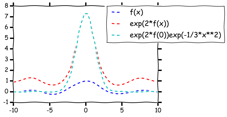
Illustration of Laplace’s method with $f(x) = \sin(x)/x$.
To understand how the integral approximation of a maximum works, let us review briefly Laplace’s method. The best is to do this in a simple case. Thus, assume that we are given a smooth function $f:[a,b]\to \R$ which has a unique maximum at $x_0\in (a,b)$, Laplace’s method to approximate $f(x_0)$ is to compute the integral
\begin{align*}
I_s \doteq \int_a^b \exp( s f(x) ) dx
\end{align*}
for some large value of $s>0$. The idea is that this behaves like a Gaussian integral. Indeed, writing $f(x) = f(x_0) + f'(x_0)(x-x_0) + \frac12 f’’(x_0) (x-x_0)^2 + R_3(x)$, since $x_0$ is a maximizer of $f$, $f'(x_0)=0$ and $-q\doteq f’’(x_0)<0$. Under appropriate technical assumptions, \begin{align*} I_s \sim \int_a^b \exp( s f(x_0) ) \exp( -\frac{(x-x_0)^2}{2/(sq)} ) \,dx \end{align*} as $s\to \infty$. Now, as $s$ gets large, $\int_a^b \exp( -\frac{(x-x_0)^2}{2/(sq)} ) \,dx \sim \int_{-\infty}^{\infty} \exp( -\frac{(x-x_0)^2}{2/(sq)} ) \,dx = \sqrt{ \frac{2\pi}{sq} }$ and hence \begin{align*} I_s \sim \exp( s f(x_0) ) \sqrt{ \frac{2\pi}{sq} }\,. \end{align*} Intuitively, the dominant term in the integral $I_s$ is $\exp( s f(x_0) )$. It should also be clear that the fact that we integrate with respect the Lebesgue measure does not matter much: We could have integrated with respect to any other measure as long as that measure puts a positive mass on the neighborhood of the maximizer. The method is illustrated on the figure shown below. The take home message of this is that if we integrate the exponential of a function that has a pronounced maximum then we can expect that the integral will be close to the exponential function of the maximum. Since $M_\lambda$ is already the exponential function of the expression to be maximized, this gives us the idea to replace $\max_\lambda M_\lambda$ with $\bar M = \int M_\lambda h(\lambda) d\lambda$ where $h$ will be conveniently chosen so that the integral can be calculated in closed form (this is not really a requirement against the method, but it just makes the argument shorter). The main benefit of replacing the maximum with an integral is of course that (from Fubini's theorem) we easily get \begin{align} \EE{ \bar M } = \int \EE{ M_\lambda } h(\lambda) d\lambda \le 1 \label{eq:barmintegral} \end{align} and thus \begin{align} \Prob{ \log(\bar M) \ge u } \le e^{-u}\,. \label{eq:barmbound} \end{align} Thus, it remains to choose $h$ and calculate $\bar M$. When choosing $h$ we want two things: $h$ should put a large mass at the maximizer of $M_\lambda$ (which is $V^{-1}Z$), and either $\bar M$ should be available in closed form (with $\bar M \approx \max_\lambda M_\lambda$ in some sense), or a lower bound on $\bar M$ should be easy to obtain which is still close to $\max_\lambda M_\lambda$. Recalling the form of $M_\lambda$, we can realize that if we choose $h$ to be the density of Gaussian then the calculation of $\bar M$ will reduce to the calculation of a Gaussian integral, a convenient outcome since Gaussian integrals can be evaluated in closed form. In particular, setting $h$ to be the density of $\mathcal N(0,H^{-1})$, we find that \begin{align*} \bar M = \frac{1}{\sqrt{(2\pi)^d \det H^{-1}}} \int \exp( \lambda^\top Z - \frac12 \norm{\lambda}_{V}^2 - \frac12 \norm{\lambda}_{H}^2 ) d\lambda\,. \end{align*} Completing the square we get \begin{align*} \lambda^\top Z - \frac12 \norm{\lambda}_{V}^2 - \frac12 \norm{\lambda}_{H}^2 & = %\frac12 \norm{Z}_{V^{-1}}^2 -\frac12 \left\{ \norm{\lambda - V^{-1}Z}_{V}^2 + \norm{\lambda}_H^2 \right\} \\ %& = %\frac12 \norm{Z}_{V^{-1}}^2 -\frac12 \left\{ \norm{\lambda-(H+V)^{-1}Z}_{H+V}^2+\norm{Z}_{V^{-1}}^2-\norm{Z}_{(H+V)^{-1}}^2 \right\} \\ %& = \frac12 \norm{Z}_{(H+V)^{-1}}^2 -\frac12 \norm{\lambda-(H+V)^{-1}Z}_{H+V}^2\,. \end{align*} Hence, a short calculation gives \begin{align*} \bar M %&= %\frac{1}{\sqrt{(2\pi)^d \det H^{-1}}} \exp( \frac12 \norm{Z}_{(H+V)^{-1}}^2 ) \int \exp( -\frac12 \norm{\lambda-(H+V)^{-1}Z}_{H+V}^2 ) d\lambda\\ %& = %\frac{1}{\sqrt{(2\pi)^d \det H^{-1}}} \exp( \frac12 \norm{Z}_{(H+V)^{-1}}^2 ) %\sqrt{(2\pi)^d \det (H+V)^{-1} }\\ & = \left(\frac{\det (H)}{\det (H+V)}\right)^{1/2} \exp( \frac12 \norm{Z}_{(H+V)^{-1}}^2 ) \,, \end{align*} which, combined with \eqref{eq:barmbound} gives \begin{align} \label{eq:selfnormalizedbound} \Prob{ \frac12 \norm{Z}_{(H+V)^{-1}}^2 \ge u+ \frac12 \log \frac{\det (H+V)}{\det(H)} } \le e^{-u}\,. \end{align} Now choosing $H=V$, we have $\det(H+V) = 2^d \det(V)$ and $\norm{Z}_{(H+V)^{-1}}^2 = \norm{Z}_{(2V)^{-1}}^2 = Z^\top (2V)^{-1} Z = \frac12 \norm{Z}_{V^{-1}}^2$, giving \begin{align*} \Prob{ \norm{Z}_{V^{-1}}^2 \ge 2\log(2)d+ 4u } \le e^{-u}\,. \end{align*} Using the identity $V^{1/2}(\hat \theta_t - \theta_*) = \norm{Z}_{V^{-1}}^2$ we get that \begin{align*} \cC_{t+1} = \left\{ \theta\in \R^d \,:\, \norm{\hat\theta_t-\theta}_V^2 \le 2\log(2)d+4 \log(\tfrac1\delta) \right\} \end{align*} is a $(1-\delta)$-level confidence set for $\theta_*$. Compared with \eqref{eq:confchi2} (the confidence set that is based on approximating the tail of the chi-square distribution using Chernoff's method), we see that the two radii scale similarly as a function of $d$ and $\delta$, with the new confidence set losing a bit (though only by a constant factor) as $\delta\to 0$. In general, the radii are incomparable. This is quite remarkable given the generality gained.
Confidence sets for sequential designs
This approach just described generalizes almost without any changes to the case when $A_1,\dots,A_t$ are not fixed, but are sequentially chosen as it is done by UCB (this is what is known as a “sequential design” in statistics). The main difference is that in this case it is not possible to choose $H=V$ in the last step. We will also drop the assumption that $V_t(0)$ is invertible and hence use $V_t(\lambda)$ with $\lambda>0$ in place of $V = V_t(0)$. Because of this, we need to replace the identity \eqref{eq:lserror0} with
\begin{align}
%\hat \theta_t
% &= V_t^{-1}(\lambda) \sum_{s=1}^t A_s A_s^\top \theta_* + V_t^{-1}(\lambda) \sum_{s=1}^t \eta_s A_s \\
% & = V_t^{-1}(\lambda) \left(\lambda I + \sum_{s=1}^t A_s A_s^\top\right) \theta_*
% + V_t^{-1}(\lambda) \sum_{s=1}^t \eta_s A_s – \lambda V_t^{-1}(\lambda)\theta_*
% & = \theta_* + V_t^{-1}(\lambda) Z – \lambda V_t^{-1}(\lambda)\theta_*
\hat \theta_t -\theta_* = V_t^{-1}(\lambda) Z – \lambda V_t^{-1}(\lambda)\theta_*\,,
\label{eq:hthdeviation}
\end{align}
and thus
\begin{align*}
V_t^{1/2}(\lambda) (\hat \theta_t -\theta_*) = V_t^{-1/2}(\lambda) Z – \lambda V_t^{-1/2}(\lambda)\theta_*\,.
\end{align*}
Inequality \eqref{eq:selfnormalizedbound} still holds, though, as already noted, in this case the choice $H=V$ is not available because this would make the density $h$ random, which would undermine the equality in \eqref{eq:barmintegral} (one may try to condition on $V$ to bound $\EE{\bar M}$ but this introduces other problems). Hence, we will simply set $H=\lambda I$, which gives a high-probability bound on $\norm{ Z }_{V_t^{-1}(\lambda)}^2$ and eventually giving rise to the following theorem:
Theorem: Assuming that $(\eta_s)_s$ are conditionally $1$-subgaussian, for any $u\ge 0$,
\begin{align}
\Prob{ \norm{\hat \theta_t – \theta_*}_{V_t(\lambda)} \ge \sqrt{\lambda} \norm{\theta_*} + \sqrt{ 2 u + \log \frac{\det V_t(\lambda)}{\det (\lambda I)} } } \le e^{-u}\,
\label{eq:ellipsoidbasic}
\end{align}
and in particular, assuming $\norm{\theta_*}\le S$,
\begin{align}
C_{t+1} = \left\{ \theta\in \R^d\,:\,
\norm{\hat \theta_t – \theta}_{V_t(\lambda)} \le \sqrt{\lambda} S + \sqrt{ 2 \log(\frac1\delta) + \log \frac{\det V_t(\lambda)}{\det (\lambda I)} } \right\}
\label{eq:ellipsoidconfset}
\end{align}
is a $(1-\delta)$-level confidence set: $\Prob{\theta_*\in C_{t+1}}\ge 1-\delta$.
Avoiding union bounds
For our results we need to ensure that $\theta_*$ is included in all of $C_1,C_2,\dots$. To ensure this one can use the union bound: In particular, we can replace $\delta$ used in the definition of $C_{t+1}$ by $\delta/(t(t+1))$. Then, the probability of none of $C_1,C_2,\dots$ containing $\theta_*$ is at most $\delta \sum_{t=1}^\infty \frac{1}{t(t+1)} = \delta$. The effect of this is that the radius of the confidence ellipsoid used in round $t$ is increased by a factor of $O(\log(t))$, which results in loser bounds and a larger regret. Fortunately, this is actually easy to avoid by resorting to a stopping time argument due to Freedman.
For developing the argument fix some positive integer $n$. To explain the technique we need to make the time dependence of $Z$ explicit. Thus, for $t\in [n]$ we let $Z_t = \sum_{s=1}^t X_s A_s$. Define also $M_\lambda(t)\doteq\exp( \lambda^\top Z_t – \frac12 \lambda^\top V_t(0) \lambda )$. In constructing $C_{t+1}$, the core inequality in the previous proof was that $\EE{ M_\lambda(t) } \le 1$ which allowed us to conclude the same for $\bar M(t) \doteq \int h(\lambda) M_\lambda(t) d\lambda$ and thus via Chernoff’s method led to $\Prob{\bar M(t) \ge e^{t}}\le e^{-t}$. As it was briefly mentioned on earlier, the proof of $\EE{ M_\lambda(t) } \le 1$ is based on chaining the inequalities
\begin{align}
\EE{ M_\lambda(s) | M_\lambda(s-1) } \le M_\lambda(s-1)
\label{eq:supermartingale}
\end{align}
for $s=t,t-1,\dots,1$, where we can define $M_\lambda(0)=1$. That $(M_\lambda(s))_s$ satisfies \eqref{eq:supermartingale} makes this sequence what is called a supermartingale adapted to the filtration $(\cF_s)_s \doteq (\sigma(A_1,X_1,\dots,A_s,X_s))_s$:
Definition (supermartingale): Let $(\cF_s)_{s\ge 0}$ be a filtration. A sequence of random variables, $(X_s)_{s\ge 0}$, is called an $(\cF_s)_s$-adapted supermartingale if $(X_s)_s$ is $(\cF_s)_s$ adapted (i.e., $X_s$ is $\cF_s$-measurable), the expectation of all the random variables is defined, and $\EE{X_s|\cF_{s-1}}\le X_{s-1}$ holds for $s=1,2,\dots$.
Integrating the above inequalities in \eqref{eq:supermartingale} with respect to $h(\lambda) d\lambda$ we immediately see that $(\bar M(s))_s$ is also an $(\cF_s)_s$ supermartingale with the filtration $(\cF_s)_s$ as before. A supermartingale process $(X_s)_s$ has the advantageous property that if we “stop it” at a random time $\tau\in [n]$ “without peeking into the future” then its mean still cannot increase: $\EE{X_\tau} \le \EE{X_1}$. When $\tau$ is a random time with this property, it is called a stopping time:
Definition (stopping time): Let $(\cF_s)_{s\in [n]}$ be a filtration. Then a random variable $\tau$ with values in $[n]$ is a stopping time given $(\cF_s)_s$ if for any $s\in [n]$, $\{\tau=s\}$ is an event of $\cF_s$.
Stopping times are after also defined when $n=\infty$ but we will not need this generality here.
Let $\tau$ be thus an arbitrary stopping time given the filtration $(\cF_s)_s \doteq (\sigma(A_1,X_1,\dots,A_s,X_s))_s$. In accordance of our discussion, $\EE{ \bar M(\tau) } \le \EE{ \bar M(0) } = 1$. From this it immediately follows that \eqref{eq:ellipsoidbasic} holds even when $t$ is replaced by $\tau$.
To see how this can be used to our advantage it will be convenient to introduce the events
\begin{align*}
\cE_t = \left\{ \norm{\hat \theta_t – \theta_*}_{V_t(\lambda)} \ge \sqrt{\lambda} S + \sqrt{ 2u + \log \frac{\det V_t(\lambda)}{\det (\lambda I)} } \right\}\,, \qquad t=1,\dots,n\,.
\end{align*}
With this, \eqref{eq:ellipsoidbasic} takes the form $\Prob{\cE_t}\le e^{-u}$ and by our discussion, for any random index $\tau\in [n]$ which is a stopping time with respect to $(\cF_t)_t$, we also have $\Prob{\cE_{\tau}} \le e^{-u}$. Now, choose $\tau$ to be the smallest round index $t\in [n]$ such that $\cE_t$ holds, or $n$ when none of $\cE_1,\dots,\cE_n$ hold. Formally, if the probability space holding the random variables is $(\Omega,\cF,\PP)$, we define $\tau(\omega) = t$ if $\omega\not \in \cE_1,\dots,\cE_{t-1}$ and $\omega \in \cE_t$ for some $t\in [n]$ and we let $\tau(\omega)=n$ otherwise. Since $\cE_1,\dots,\cE_t$ are $\cF_t$ measurable, $\{\tau=t\}$ is also $\cF_t$ measurable. Thus $\tau$ is a stopping time with respect to $(\cF_t)_t$. Now, consider the event
\begin{align*}
\cE= \left\{ \exists t\in [n] \mathrm{ s.t. } \norm{\hat \theta_t – \theta_*}_{V_t(\lambda)} \ge \sqrt{\lambda} S + \sqrt{ 2u + \log \frac{\det V_t(\lambda)}{\det (\lambda I)} } \right\}\,.
\end{align*}
Clearly, if $\omega\in \cE$ then $\omega \in \cE_{\tau}$. Hence, $\cE\subset \cE_{\tau}$ and $\Prob{\cE}\le \Prob{\cE_{\tau}}\le e^{-u}$. Finally, since $n$ was arbitrary we also get that the upper limit on $t$ in the definition of $\cE$ can be removed. This shows that the bad event that any of the confidence sets $C_{t+1}$ of the previous theorem fail to hold the parameter vector $\theta_*$ is also bounded by $\delta$:
Corollary (Uniform bound):
\begin{align*}
\Prob{ \exists t\ge 0 \text{ such that } \theta_*\not\in C_{t+1} } \le \delta\,.
\end{align*}
Recalling \eqref{eq:hthdeviation}, for future reference we now restate the conclusion of our calculations in a form concerning the tail of the process $(Z_s)_s \doteq (\sum_{s=1}^t \eta_s A_s)_s$:
Corollary (Uniform self-normalized tail bound on $(Z_s)_s$): For any $u\ge 0$,
\begin{align*}
\Prob{ \exists t\ge 0 \text{ such that }
\norm{Z_t}_{V_t^{-1}(\lambda)} \ge \sqrt{ 2u + \log \frac{\det V_t(\lambda)}{\det (\lambda I)} }
} \le e^{-u}\,.
\end{align*}
Putting things together: The regret of Ellipsoidal-UCB
We will call the version of UCB that uses the confidence set of the previous section the “Ellipsoidal-UCB”. To state a bound on the regret of Ellipsoidal-UCB, let us summarize the conditions we will need: Recall that $\cF_t = \sigma(A_1,X_1,\dots,A_{t-1},X_{t-1},A_t)$, $X_t = \ip{A_t,\theta_*}+\eta_t$ and $\cD_t\subset \R^d$ is the action set available at the beginning of round $t$. We will assume that the following hold true:
- $1$-subgaussian martingale noise: $\forall \lambda\in \R$, $s\in \N$, $\EE{\exp(\lambda \eta_s)|\cF_{s} } \le \exp(\frac{\lambda^2}{2})$.
- Bounded parameter vector: $\norm{\theta_*}\le S$
- Bounded actions: $\sup_{t} \sup_{a\in \cD_t} \norm{a}_2\le L$
- Bounded mean reward: $|\ip{a,\theta_*}|\le 1$ for any $a\in \cup_t \cD_t$
Combining our previous results gives the following corollary:
Theorem (Regret of Ellipsoidal-UCB): Assume that the conditions listed above hold. Let $\hat R_n = \sum_{t=1}^n \max_{a\in \cD_t} \ip{a,\theta_*} – \ip{A_t,\theta_*}$ be the pseudo-regret of the Ellipsoidal-UCB algorithm that uses the confidence set \eqref{eq:ellipsoidconfset} in round $t+1$. With probability $1-\delta$, simultaneously for all $n\ge 1$,
\begin{align*}
R_n
\le \sqrt{ 8 d n \beta_{n-1} \, \log \frac{d\lambda+n L^2}{ d\lambda } }\,,
\end{align*}
where
\begin{align*}
\beta_{n-1}^{1/2}
& = \sqrt{\lambda} S + \sqrt{ 2\log(\frac1\delta) + \log \frac{\det V_{n-1}(\lambda)}{\det (\lambda I)}} \\
& \le \sqrt{\lambda} S + \sqrt{ 2\log(\frac1\delta) \,+\,\frac{d}{2}\ \log\left( 1+n \frac{L^2}{ d\lambda }\right)} \,.
\end{align*}
Choosing $\delta = 1/n$, $\lambda = \mathrm{const}$ we get that $\beta_n^{1/2} = O(d^{1/2} \log^{1/2}(n/d))$ and thus the expected regret of Ellipsoidal-UCB, as a function of $d$ and $n$ satisfies
\begin{align*}
R_n
& = O( \beta_n^{1/2} \sqrt{ dn \log(n/d) } )
= O( d \log(n/d) \sqrt{ n } )\,.
\end{align*}
Note that this holds simultaneously for all $n\in \N$. We also see that (apart from logarithmic factors) the regret scales linearly with the dimension $d$, while it is completely free of the cardinality of the action set $\cD_t$. Later we will see that this is indeed unavoidable in general.
Fixed action set
When the action set is fixed and small, it is better to construct the upper confidence bounds for the payoffs of the actions directly. This is best illustrated for the fixed-design case when $A_1,\dots,A_t$ are deterministic, the noise is i.i.d. standard normal and the Grammian is invertible even with $\lambda=0$. In this case, the confidence set for $\theta_*$ was given by \eqref{eq:confchi2}, i.e., the radius is $\beta_t = 2d+8\log(1/\delta)$. By our earlier observation (see here),
\begin{align*}
\UCB_{t+1}(a) = \ip{a,\hat \theta_t} + (2d+8\log(1/\delta))^{1/2} \norm{a}_{V_t^{-1}}\,.
\end{align*}
Notice that the “radius” $\beta_t$ scales linearly with $d$, which then propagates into the UCB values. By our main theorem, this then propagates into the regret bound making the regret scale linearly with $d$. It is easy to see that the linear dependence of $\beta_t$ is an unavoidable consequence of using the confidence set construction which relied on the properties of the chi-square distribution with $d$ degrees of freedom. Unfortunately, this means that even when $\cD_t = \{e_1,\dots,e_d\}$, corresponding to the standard finite-action stochastic bandit case, the regret will scale linearly with $d$ (the number of actions), whereas we have seen it earlier that the optimal scaling is $\sqrt{d}$. To get this scaling we thus see that we need to avoid a confidence set construction which is based on ellipsoids.
A simple construction which avoids this problem is as follows: Staying with the fixed design and independent Gaussian noise, recall that $\hat \theta_t – \theta_* = V^{-1} Z \sim \mathcal N(0,I)$ (cf. \eqref{eq:standardnormal}). Fix $a\in \R^d$. Then, $\ip{a, \hat \theta_t – \theta_*} = a^\top V^{-1} Z \sim \mathcal N(0, \norm{a}_{V^{-1}}^2)$. Hence, by the subgaussian property of Gaussians, defining
\begin{align}\label{eq:lingaussianperarmucb}
\mathrm{UCB}_{t+1}(a) = \ip{a,\hat \theta_t} + \sqrt{ 2 \log(1/\delta) }\, \norm{a}_{V_t^{-1}} \,
\end{align}
we see that $\Prob{ \ip{a,\theta_*}>\mathrm{UCB}_{t+1}(a) } \le \delta$. Note that this bound indeed removed the extra $\sqrt{d}$ factor.
Unfortunately, the generalization of this method to the sequential design case is not obvious. The difficulty comes from controlling $\ip{a, V^{-1} Z}$ without relying on the exact distributional properties of $Z$.
Notes
An alternative to the $2$-norm based construction is to use $1$-norms. In the fixed design setting, under the independent Gaussian noise assumption, using Chernoff’s method this leads to
\begin{align}
\cC_{t+1} = \left\{ \theta\in \R^d\,:\, \norm{ V^{1/2}(\hat \theta_t-\theta) }_1 \le
\sqrt{2 \log(2) d^2 +2d \log(1/\delta) }
\right\}\,.
\label{eq:confl1}
\end{align}
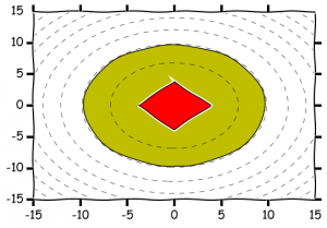
Illustration of 2-norm and 1-norm based confidence sets in 2 dimension with $\delta=0.1$, $\hat \theta_t=0$, $V=I$.
References
As mentioned in the previous post, the first paper to consider UCB-style algorithms is by Peter Auer:
- Peter Auer: Using confidence bounds for exploitation-exploration trade-offs. The Journal of Machine Learning Research. 3:397-422, 2002.
The setting of the paper is the one when in every round the number of actions is bounded by a constant $K>0$. For this setting an algorithm (SupLinRel) is given and it is shown that its expected regret is at most $O(\sqrt{ d n \log^3(K n \log(n) ) })$, which is better by a factor of $\sqrt{d}$ than the bound derived here, but it also depends on $K$ (although only logarithmically) and is slightly worse than the bound shown here in its dependence on $n$, too. The dependence on $K$ can be traded for the dependence on $d$ by considering an $L/\sqrt{n}$-cover of the ball $\{ a\,:\, \norm{a}_2 \le L \}$, which gives $K = \Theta( (\sqrt{n}/L)^d )$ and a regret of $O(d^2 \sqrt{n \log^3(n)})$ for $n$ large, which is larger than the regret given here. Note that SupLinRel can also be run without actually discretizing the action set, just its confidence intervals have to be set based on the cardinality of the discretization (in particular, inflated by a factor of $\sqrt{d}$).
SupLinRel builds on LinRel, which, as we noted, is UCB with a specific upper confidence value. LinRel uses confidence bounds of the form \eqref{eq:lingaussianperarmucb} with a confidence parameter roughly of the size $\delta = 1/(n \log(n) K)$. This is possible because SupLinRel uses LinRel in a nontrivial way, “filtering” the data that LinRel works on.
In particular, SupLinRel uses a version of the “doubling trick”. The main idea is to keep at most $\log_2(n^{1/2})$ lists that hold mutually exclusive data. In every round SupLinRel starts with list of index $s=1$ and feeds the data of this list to LinRel which calculates UCB values and confidence width based on the data it received. If all the calculated widths are small (below $\theta=n^{-1/2}$) then the action with the highest UCB value is selected and the data generated is thrown away. Otherwise, if any width is above $2^{-s}$ then the corresponding action is chosen and the data observed is added to the list with index $s+1$. If all the widths are below $2^{-s}$ then all actions which, based on the current confidence intervals calculated by LinRel, cannot be optimal are eliminated, $s$ is incremented and the process is repeated until an action is chosen. Overall the effect of this is that the lists grow, lists with smaller index growing first until they are sufficiently rich for their desired target accuracy. Furthermore, the contents of a list is determined not by data of the list but by data on lists with smaller index. Because of this, the fixed-design confidence interval design as described here can be used, which ultimately saves the $O(\sqrt{d})$ factor. While apart from log-factors SupLinRel is unimprovable, in practice SupLinRel is excessively wasteful.
A confidence ellipsoid construction based on covering arguments can be found in the paper by Varsha Dani, Thomas Hayes and Sham Kakade:
- V. Dani, T. Hayes and S. Kakade: Stochastic Linear Optimization under Bandit Feedback, COLT-2008.
An analogous construction is given by
- Paat Rusmevichientong, John N. Tsitsiklis: Linearly Parameterized Bandits, MOR, 35:395-411
The confidence ellipsoid construction described in this post is based on
- Yasin Abbasi-Yadkori, Dávid Pál and Csaba Szepesvári: Improved Algorithms for Linear Stochastic Bandits, NIPS, pp. 2312-2320, 2011.
Laplace’s method is also called the “Method of Mixtures” in the probability literature and it’s use goes back to the work of Robbins and Siegmund that was done in 1970. In practice, the improvement that results from using Laplace’s method as compared to the previous ellipsoidal constructions that are based on covering arguments is quite enormous.
As mentioned earlier, a variant of SupLinRel that is based on ridge regression (as opposed to LinRel, which is based on truncating the smallest eigenvalue of the Grammian) is described in
- Wei Chu, Lihong Li, Lev Reyzin, Robert E. Schapire: Contextual Bandits with Linear Payoff Functions, AISTATS, pp. 208-214, 2011.
The algorithm, which is called SupLinUCB, uses the same construction as SupLinRel and enjoys the same regret.
For a fixed action set (i.e., when $\cD_t=\cD$), one can use an elimination based algorithm, which in every phase collects data by using a “spanning set” of the remaining actions. At the end of the phase, since the data collected in the phase only depends on data collected in previous phases, one can use Hoeffding’s bounds to construct UCB values for the actions. This is the idea underlying the “SpectralEliminator” algorithm in the paper
- Michal Valko, Remi Munos, Branislav Kveton and Tomas Kocak: Spectral Bandits for Smooth Graph Functions, ICML 2014.

Thanks for sharing the posts. I have gained a lot of insights! Hope to finish all soon:) Just to point out there is repeat in Notes session.
Thank you Dr. Lattimore. I have a question about the derivation of the inequality after (6), where in the bracket, you said first let s=n, and then s=n-1,etc. But what is n? is it s=t instead?
Hi!
Thanks for the comment. You are right: $n$ should have been $t$ here. Oh, and I edited the page to reflect this.
– Csaba
Hi,
Thanks a lot for your great blog and book!
I was reading Exercise 20.12 in the book on the sequential likelihood ratio confidence set extracted from Lemma 2 of Lai and Robbins (1985). This construction seems to be for the iid bandit. Can it be generalized to linear bandit as well?
Hi Claire,
Yes, this result holds very generally. Only a martingale structure is being used and even the estimates can be any appropriately measurable function.
Thanks for your reply!
Could you kindly point out a reference for the general setting, or briefly mention what the corresponding martingale is in the general setting?
Hi,
To derive equation (1), do we need some additional assumptions on the choice of $a_s$ (e.g. they form a basis)?
Best,
Zeyad Emam
Yes. It is assumed that V is non-singular, which is possible only when $(a_s)$ span $\R^d$.