
Recall that in the adversarial contextual $K$-action bandit problem, at the beginning of each round $t$ a context $c_t\in \Ctx$ is observed. The idea is that the context $c_t$ may help the learner to choose a better action. This led us to change the benchmark in the definition of regret. In this post we start with reviewing how contextual bandit problems can be defined in the stochastic setting. We use this setting to motivate the introduction of stochastic linear bandits, a fascinatingly rich model with much structure and which will be the topic of a few of the next posts. Besides defining stochastic linear bandits we also cover how UCB can be generalized to this setting.
Stochastic contextual bandits
In the standard $K$-action stochastic contextual bandit problem at the beginning of round $t$ the learner observes a context $C_t\in \Ctx$. The context may or may not be random. Next, the learner chooses its action $A_t\in [K]$ based on the information available. So far these is no difference to the adversarial setting. The difference comes from the assumption that the reward $X_t$ which is incurred satisfies
\begin{align*}
X_t = r(C_t,A_t) + \eta_t\,,
\end{align*}
where $r:\Ctx\times [K]\to \R$ is the so-called reward function, which is unknown to the learner, while $\eta_t$ is random noise.
In particular, the assumption on the noise is as follows: Let
\begin{align*}
\cF_t = \sigma(C_1,A_1,X_1,\dots,C_{t-1},A_{t-1},X_{t-1},C_t,A_t)
\end{align*}
be the $\sigma$-field summarizing the information available just before $X_t$ is observed. Then, given the past, we assume that $\eta_t$ is conditionally $1$-subgaussian:
\begin{align*}
\EE{ \exp( \lambda \eta_t ) | \cF_t } \le \exp(\frac{\lambda^2}{2})\,.
\end{align*}
(The constant $1$ is chosen to minimize the number of symbols; there is no difficulty considering the more general case of conditionally $\sigma^2$-subgaussian noise.) As discussed beforehand, subgaussian random variables have zero mean, hence the above assumption also implies that $\EE{\eta_t|\cF_t}=0$, or $\EE{X_t|\cF_t}=r(C_t,A_t)$. In words, for any given $(c,a)\in \Ctx\times [K]$ context-action pair, $r(c,a)$ gives the mean reward of action $a$ in context $c$.
If $r$ was given then the learner wishing to maximize the total expected reward would choose the action $A_t^* = \argmax_{a\in [K]} r(C_t,a)$ in round $t$ (if multiple maximizers exist, choose one). The loss due to the lack of knowledge of $r$ makes the learner incur the (expected) regret
\begin{align*}
R_n = \EE{ \sum_{t=1}^n \max_{a\in[K]} r(C_t,a) – \sum_{t=1}^n X_t }\,.
\end{align*}
Towards linear bandits
To act eventually optimally, the learner may estimate $r(c,a)$ for each $(c,a)\in \Ctx\times [K]$ pair. Similarly to what happens in the adversarial setting, this is ineffective when the number of context-action pairs is large in that in this case the regret can be very high for a long time. In particular, just like in the adversarial case the worst-case regret over all possible contextual problems with $M$ contexts and mean reward in $[0,1]$ is at least $\Omega( \sqrt{nMK} )$. One refinement of the bound is to replace $M$ by the number of effective contexts, i.e., contexts that appear frequently. But if context has a lot of detailed information, this still may very high. However, if the reward function enjoys additional structure, this worst case argument will fail. The additional structure may come in many different forms. “Smoothness”, which was also mentioned previously when we discussed adversarial contextual bandits, is one example.
An alternative (but related) assumption uses the linear structure of the set $\R^{\Ctx\times [K]}$ of all possible reward functions (recall that real-valued functions form a vector space over the reals). The so-called linearity assumption postulates that $r$ belongs to a low-dimensional linear subspace $\cS$ of $\cV \doteq \R^{\Ctx\times [K]}$.
A somewhat finer condition is to assume a specific “parameterization” of the subspace $\cS$. This works as follows: It is assumed that the learner is given access to a map $\psi: \Ctx \times [K] \to \R^d$ and that with some unknown parameter vector $\theta_*\in \R^d$,
\begin{align*}
r(c,a) = \theta_*^\top \psi(c,a)\,, \qquad \forall (c,a)\in \Ctx\times [K]\,.
\end{align*}
The map $\psi$, in line with the machine learning literature, is called a feature-map. Assuming the knowledge of $\psi$ is equivalent to knowing the linear subspace $\cS$. The refinement of the subspace condition comes from extra assumptions that one puts on $\theta_*$, such as that the magnitude of $\theta_*$ as measured in a certain norm $\norm{\cdot}$ is “small”, or that even $\norm{\theta_*}\le B$ with $B$ known, or, more generally, that $\theta_*\in \Theta$ for some known (small) set $\Theta\subset \R^d$ or a mix of these.
The idea of feature maps is best illustrated with an example: If the context denotes the visitor of a website selling books, the actions are books to recommend, the reward is the revenue on a book sold then the features could indicate the interests of the visitors as well as the domain and topic of the books. If the visitors and books are assigned to finitely many categories, indicator variables of all possible combinations of these categories could be used to create the feature map. Of course, many other possibilities exist. One such possibility is to train a neural network (deep or not) on historical data to predict the revenue and use the nonlinear map that we obtained by removing the last layer of the neural network. The subspace $\Psi$ spanned by the feature vectors $\{\psi(c,a)\}_{c,a}$ in $\R^d$ is called the feature-space.
An assumption on $\norm{\theta_*}$ encodes smoothness of $r$. In particular, from Hölder’s inequality,
\begin{align*}
|r(c,a)-r(c’,a’)| \le \norm{\theta_*} \norm{\psi(c,a)-\psi(c’,a’)}_*\,,
\end{align*}
where $\norm{\cdot}_*$ denotes the dual of $\norm{\cdot}$. This is how $\psi$ implicitly encodes “smoothness”. Restrictions on $\norm{\theta_*}$ have a similar effect to assuming that the dimensionality $d$ of the subspace $\cS$ is small. In fact, one may push this to the extreme and allow $d$ to be infinite, which can buy tremendous flexibility. With this much flexibility the linearity assumption perhaps feels less limiting.
Another assumption which is similar yet different from the previously mentioned ones is to assume that $\theta_*$ is sparse. By this we mean that many entries of $\theta_*$ are zero. Sometimes this is written as that the $0$-norm of $\theta_*$ is small. Here, the zero-norm, $\norm{\theta_*}_0$, just counts the number of nonzero entries of $\theta_*$: $\norm{\theta_*}_0 = |\{ i \,:\, \theta_{*,i}\ne 0 \}|$. The point of the sparsity assumption is to remove the burden from the designer of the feature map to leave out components that are unnecessary to get a good approximation of $r$: The designer may then include any component that may be relevant in predicting the reward, enforcing the selection of the “relevant” features by imposing a constraint on the number of nonzero entries of $\theta_*$.
Stochastic linear bandits
Stochastic linear bandits arise from realizing that when the reward is linear in the feature vectors, the identity of the actions becomes secondary and we rather let the algorithms choose the feature vectors directly: the identity of the actions adds no information or structure to the problem. This results in the following model: In round $t$, the learner is given the decision set $\cD_t\subset \R^d$ that it has to choose an action from. If the learner chooses $A_t\in \cD_t$, it incurs the reward
\begin{align*}
X_t = \ip{A_t,\theta_*} + \eta_t\,,
\end{align*}
where $\eta_t$ is $1$-subgaussian given $\cD_1,A_1,X_1,\dots,\cD_{t-1},A_{t-1},X_{t-1},\cD_t$ and $A_t$. The regret suffered is
\begin{align*}
R_n = \EE{ \sum_{t=1}^n \max_{a\in \cD_t} \ip{a,\theta_*} – \sum_{t=1}^n X_t }\,.
\end{align*}
With $\cD_t = \{ \phi(c_t,k) \,:\, k\in [K] \}$ the model reproduces contextual bandits. When $\cD_t = \{e_1,\dots,e_d\}$ (where $e_1,\dots,e_d$ are the unit vectors in the standard Euclidean basis), stochastic linear bandits reproduce finite action stochastic bandits. Linear stochastic bandits also arise naturally with combinatorial action sets, i.e., when $\cD \subset \{0,1\}^d$: Many combinatorial problems (such as matching, least-cost problems in directed graphs, choosing spanning trees, etc.) can be written as linear optimization over some combinatorial set $\cD$ obtained from considering incidence vectors often associated with some graph. We hope to cover some of these fun problems later.
UCB for linear bandits
The UCB algorithm is a very attractive algorithm for finite-action stochastic bandits: It is near-minimax optimal and is also almost instance optimal for any finite horizon and even asymptotically. It is thus quite natural to attempt to generalize UCB to the linear settings.
The generalization is based on the view that UCB implements the optimism in the face of uncertainty principle, according to which one should choose the actions as if the environment (in our case the linear bandit environment) was as nice as plausible possible. In finite-action stochastic bandit problems the principle dictates to choose the action with the largest upper confidence bound. In the case of linear bandit problems this still holds, but now to calculate the upper confidence bounds one should also better take into account the information conveyed by all the rewards observed because all the data $(A_1,X_1,\dots,A_{t-1},X_{t-1})$ is now connected through the unknown parameter vector.
One idea is to construct a “confidence set” $\cC_{t}$ based on $(A_1,X_1,\dots,A_{t-1},X_{t-1})$ that contains the unknown parameter vector $\theta_*$ with high probability. Leaving details of how the confidence set is constructed aside for a moment but assuming that the confidence set indeed contains $\theta_*$, for any given action $a\in \R^d$,
\begin{align}
\mathrm{UCB}_t(a) = \max_{\theta\in \cC_t} \ip{a,\theta}
\label{eq:UCBCt}
\end{align}
will be an upper bound on the mean payoff of $a$. The UCB algorithm that uses the confidence set $\cC_t$ at time $t$ then selects
\begin{align}
A_t = \argmax_{a\in \cD_t} \mathrm{UCB}_t(a)\,.
\label{eq:UCBgencDt}
\end{align}
In fact, the last equation is what we will take as the definition of UCB regardless of how the $\UCB_t(\cdot)$ values are defined. Of course the naming is justified only when the UCB values are indeed upper bounds on the mean payoffs of the actions.
Depending on the authors, UCB applied to linear bandits is known by many names, including but not limited to LinRel (after perhaps Linear Reinforcement Learning), LinUCB (an obvious choice), and OFUL (Optimism in the Face of Uncertainty for Linear bandits), just to mention a few.
Computation
Note that as long as $\cD_t$ has a few vectors in it, and the linear optimization problem \eqref{eq:UCBCt} can be efficiently solved (such as when $\cC_t$ convex), the computation is efficient. To discuss the computation cost further note that the computation of $A_t$ can also be written as
\begin{align}
(A_t,\tilde \theta_t) = \argmax_{(a,\theta)\in \cD_t\times \cC_t} \ip{a,\theta}\,.
\label{eq:UCBgenjoint}
\end{align}
This is a bilinear optimization problem over the set $\cD_t \times \cC_t$. In general, nothing much can be said about the computational efficiency of solving this problem. One special case when a solution can be found efficiently is when (i) the linear optimization problem $\max_{a\in \cD} \ip{a,\theta}$ can be efficiently solved for any $\theta$ (this holds in many combinatorial settings) and (ii) $\cC_t$ is the convex hull of a handful of vertices: $\cC_t = \mathrm{co}(c_{t1},\dots,c_{tp})$. Indeed, in this case for any $a\in \cD_t$, $\argmax_{\theta\in \cC_t} \ip{a,\theta}$ is one of $c_{t1},\dots,c_{tp}$. Hence, the solution to \eqref{eq:UCBgenjoint} can be obtained by solving $\max( \max_{a\in \cD_t} \ip{a,c_{t1}}, \dots, \max_{a\in \cD_t} \ip{a,c_{tp}} )$. A special case of this is when $\cC_t$ is the skewed and shifted $\ell^1$-ball, i.e. when for some nonsingular matrix $A$ and vector $\theta_0\in \R^d$, $\cC_t = \{ \theta\,:\, \norm{A(\theta – \theta_0)}_1 \le \beta_t \}$. Note that in this case $p=2d$.
Another notable case is when $\cC_t$ is an ellipsoid. To minimize clutter in writing the definition of an ellipsoid, let us introduce the notation $\norm{x}^2_V$ which is defined for a $V$ $d\times d$ positive definite matrix and its value is $x^\top V x$. The notation is justified since $\norm{\cdot}_{V}$ is indeed a norm. We will call $\norm{x}_V$ the $V$-norm of $x$. With this, choosing some center $\hat \theta\in \R^d$, $V\succ 0$ positive definite matrix and “radius” $\beta$, an ellipsoidal confidence set takes the form $\cC_t = \{\theta\in \R^d \,:\, \norm{\theta-\hat \theta}^2_{V}\le \beta \}$ (in general, $\hat \theta$, $V$ and $\beta$ will be dependent on past observations, and the reason of not absorbing $\beta$ into the definition of $V$ will become clear later).
When $\cC_t$ is of this ellipsoidal form, the UCB values are particularly simple. To see this, first we rewrite $\cC_t$ into an alternate, equivalent form. Defining $B_2 = \{x\in \R^d\,:\, \norm{x}_2\le 1\}$ to be the unit ball with respect to the Euclidean norm, it is easy to see that $\cC_t = \hat \theta + \beta^{1/2} V^{-1/2} B_2$. Using this, a short direct calculation gives
\begin{align}\label{eq:linucb}
\mathrm{UCB}_t(a) = \ip{a,\hat \theta} + \beta^{1/2} \norm{a}_{V^{-1}}\,.
\end{align}
Note the similarity to the standard finite-action UCB algorithm: Interpreting $\hat \theta$ as the estimate of $\theta_*$, $\ip{a,\hat \theta}$ can be seen as the estimate of the mean reward of $a$, while $\beta^{1/2} \norm{a}_{V^{-1}}$ is a bonus term. As we shall see later the confidence values could be defined by setting $\hat \theta$ to be the least–squares estimator (LSE) of $\theta_*$ with perhaps an appropriate regularization, while $V$ could be set to $V_t$, the “regularized Grammian” matrix defined using
\begin{align}
V_t=V_0 + \sum_{s=1}^{t} A_s A_s^\top, \qquad t\in [n]\,,
\label{eq:linbanditreggrammian}
\end{align}
where $V_0\succ 0$ is a fixed positive semidefinite matrix, which is often set to $\lambda I$ with some $\lambda>0$ tuning parameter.
When $\cD_t = \{e_1,\dots,e_d\}$ for all $t\in [n]$, $\hat \theta_i$ becomes the empirical mean of action $e_i$ (which could in this case be meaningfully called the $i$th action), while with $V_0=0$ the matrix $V_t$ is diagonal with its $i$ diagonal entry being the number of times action $e_i$ is used up to and including round $t$.
Soon we will see why the choice of $(V_t)_t$ is natural. The impatient reader may check that in the special case when $\eta_t$ is an i.i.d. zero-mean Gaussian sequence and the vectors $(A_t)_t$ are deterministically chosen (which is clearly far from what happens in UCB), $V_t$ with $V_0=0$ comes up naturally when defining a confidence set for $\theta_*$. The behavior of UCB is illustrated on the figure below.
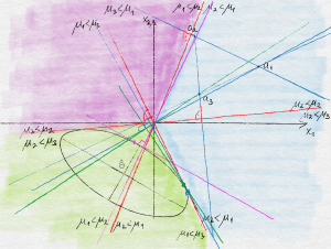
Illustration of the behavior of UCB. Three actions, labeled $a_1$, $a_2$ and $a_3$ live in the positive quadrant of $\R^2$. The plane, which also hosts $\theta_*$ is colored based on the identity of the optimal action as a function of where $\theta_*$ is. A confidence ellipsoid with center $\hat \theta$ is also shown as are the locations of the parameter vectors that give rise to the highest value for each of the actions. Action $a_1$ happens to have the highest UCB value.
A Generic Bound on the Regret of UCB
In this section we bound the regret of UCB as a function of the width of the confidence intervals used by UCB without explicitly specifying how the confidence bounds are constructed, though we make a specific assumption about the form of the width. Later we will specialize this result to two different settings. In particular, our assumptions are as follows:
- Bounded scalar mean reward: $|\ip{a,\theta_*}|\le 1$ for any $a\in \cup_t \cD_t$;
- Bounded actions: for any $a\in \cup_t \cD_t$, $\norm{a}_2 \le L$;
- Honest confidence intervals: With probability $1-\delta$, for all $t\in [n]$, $a\in \cD_t$, $\ip{a,\theta_*}\in [\UCB_t(a)-2\sqrt{\beta_{t-1}} \norm{a}_{V_{t-1}^{-1}},\UCB_t(a)]$ where $(V_{t})_t$ are given by \eqref{eq:linbanditreggrammian}.
Note that the half-width $\sqrt{\beta_{t-1}} \norm{a}_{V_{t-1}^{-1}}$ used in the assumption is the same as one gets when a confidence set $\cC_t$ is used which satisfies
\begin{align}
\cC_t \subset
\cE_t \doteq \{ \theta \in \R^d \,:\,
\norm{\theta-\hat \theta_{t-1}}_{ V_{t-1}}^2 \le \beta_{t-1} \}\,
\label{eq:ellconf}
\end{align}
with some $\hat \theta_{t-1}\in \R^d$.
Our first main result is as follows:
Theorem (Regret of UCB for Linear Bandits): Let the conditions listed above hold. Further, assume that $(\beta_t)_t$ is nondecreasing and $\beta_{n-1}\ge 1$. Then, with probability $1-\delta$, the pseudo-regret $\hat R_n = \sum_{t=1}^n \max_{a\in \cD_t} \ip{a,\theta_*} – \ip{A_t,\theta_*}$ of UCB as defined by \eqref{eq:UCBgenjoint} satisfies
\begin{align*}
\hat R_n
\le \sqrt{ 8 n \beta_{n-1} \, \log \frac{\det V_{n}}{ \det V_0 } }
\le \sqrt{ 8 d n \beta_{n-1} \, \log \frac{\trace(V_0)+n L^2}{ d\det^{1/d} V_0 } }\,.
\end{align*}
Note that the condition on $(\beta_t)_t$ is not really restrictive because we can always arrange for it to hold at the price of increasing $\beta_1,\dots,\beta_n$. We also see from the result that to get an $\tilde O(\sqrt{n})$ regret bound one needs to show that $\beta_n$ has a polylogarithmic growth (here, $\tilde O(f(n))$ means $O( \log^p(n) f(n) )$ with some $p>0$). We can also get a bound on the (expected) regret $R_n$ if $\delta\le c/\sqrt{n}$ by combining the bound of the theorem with $\hat R_n \le 2n$, which follows from our assumption that the magnitude of the immediate reward is bounded by one.
Proof: It suffices to prove the bound on the event when the confidence intervals contain the expected rewards of all the actions available in all the respective rounds. Hence, in the remainder of the proof we will assume that this holds. Let $r_t = \max_{a\in \cD_t} \ip{a,\theta_*} – \ip{A_t,\theta_*}$ be the immediate pseudo-regret suffered in round $t\in [n]$.
Let $A_t^* = \argmax_{a\in \cD_t} \ip{a,\theta_*}$ be an optimal action for round $t$. Thanks to the choice of $A_t$, $\ip{A_t^*,\theta_*}\le \UCB_t(A_t^*) \le \UCB_t(A_t)$. By assumption $\ip{A_t,\theta_*}\ge \UCB_t(A_t)-2\beta_{t-1}^{1/2} \norm{A_t}_{V_{t-1}^{-1}}$. Combining these inequalities we get
\begin{align*}
r_t \le 2 \sqrt{\beta_{t-1}} \norm{A_t}_{V_{t-1}^{-1}}\,.
\end{align*}
By the assumption that the mean absolute reward is bounded by one we also get that $r_t\le 2$. This combined with $\beta_n \ge \max(\beta_t,1)$ gives
\begin{align*}
r_t
& \le 2 \wedge 2 \sqrt{\beta_{t-1}} \norm{A_t}_{V_{t-1}^{-1}}
\le 2 \sqrt{\beta_{n-1}} (1 \wedge \norm{A_t}_{V_{t-1}^{-1}})\,,
\end{align*}
where, as before, $a\wedge b = \min(a,b)$.
Jensen’s inequality, or Cauchy-Schwarz gives $R_n \le \sqrt{n \sum_t r_t^2 }$. So it remains to bound $\sum_t r_t^2$. This is done by applying the following technical lemma:
Lemma (Elliptical Potential): Let $x_1,\dots,x_n\in \R^d$, $V_t = V_0 + \sum_{s=1}^t x_s x_s^\top$, $t\in [n]$, $v_0 = \trace(V_0)$ and $L\ge \max_t \norm{x_t}_2$. Then,
\begin{align*}
\sum_{t=1}^n 1 \wedge \norm{x_t}_{V_{t-1}^{-1}}^2 \le 2 \log \frac{\det V_{n}}{\det V_0} \le d \log \frac{v_0+n L^2}{d\det^{1/d} V_0}\,.
\end{align*}
The idea underlying the proof of this lemma is to first use that $u\wedge 1 \le 2 \ln(1+u)$ and then use an algebraic identity to prove that the sum of the logarithmic terms is equal to $\log \frac{\det V_n}{\det V_0}$. Then one can bound $\log \det V_{n}$ by noting that $\det V_{n}$ is the product of the eigenvalues of $V_{n}$, while $\trace V_{n}$ is the sum of the eigenvalues and then using the AM-GM inequality. The full proof is given at the end of the post.
Applying the bound and putting everything together gives the bound stated in the theorem.
QED.
In the next post we will look into how to construct tight ellipsoidal confidence sets. The theorem just proven will then be used to derive a regret bound.
Proof of the Elliptical Potential Lemma
Recall that we want to prove that
\begin{align*}
\sum_{t=1}^n 1 \wedge \norm{x_t}_{V_{t-1}^{-1}}^2 \le 2 \log \frac{\det V_{n}}{\det V_0} \le d \log \frac{v_0+n L^2}{d\det^{1/d} V_0}\,.
\end{align*}
where $x_1,\dots,x_n\in \R^d$, $V_t = V_0+\sum_{s=1}^t x_s x_s^\top$, $t\in [n]$, $v_0=\trace V_0$, and $\max_t \norm{x_t}_2\le L$ (cf. here).
Using that for any $u\in [0,1]$, $u \wedge 1 \le 2 \ln(1+u)$, we get
\begin{align*}
\sum_{t=1}^n 1 \wedge \norm{x_t}_{V_{t-1}^{-1}}^2 \le 2 \sum_t \log(1+\norm{x_t}_{V_{t-1}^{-1}}^2)\,.
\end{align*}
Now, we argue that this last expression is $\log \frac{\det V_{n}}{\det V_0}$. For $t \ge 1$ we have $V_{t} = V_{t-1} + x_t x_t^\top = V_{t-1}^{1/2}(I+V_{t-1}^{-1/2} x_t x_t^\top V_{t-1}^{-1/2}) V_{t-1}^{1/2}$. Hence, $\det V_t = \det(V_{t-1}) \det (I+V_{t-1}^{-1/2} x_t x_t^\top V_{t-1}^{-1/2})$. Now, it is easy to check that the only eigenvalues of $I + y y^\top$ are $1+\norm{y}_2$ and $1$ (this is because this matrix is symmetric, hence its eigenvectors are orthogonal to each other and $y$ is an eigenvector). Putting things together we see that $\det V_{n} = \det (V_0) \prod_{t=1}^{n} (1+ \norm{x_t}^2_{V_{t-1}^{-1}})$, which is equivalent to the first inequality that we wanted to prove. To get the second inequality note that by the AM-GM inequality, $\det V_n = \prod_{i=1}^d \lambda_i \le (\frac1d \trace V_n)^d \le ((v_0+n L^2)/d)^d$, where $\lambda_1,\dots,\lambda_d$ are the eigenvalues of $V_n$.
References
The literature of linear bandits is rather large. Here we restrict ourselves to the works most relevant to this post.
Stochastic linear bandits were introduced into the machine learning literature by Abe and Long:
- Naoki Abe, Alan W. Biermann, and Philip M. Long. Reinforcement learning with immediate rewards and linear hypotheses. Algorithmica, 37(4):263-293, 2003.
(An earlier version of this paper from 1999 can be found here.)
The first paper to consider UCB-style algorithms is by Peter Auer:
- Peter Auer: Using confidence bounds for exploitation-exploration trade-offs. The Journal of Machine Learning Research. 3:397-422, 2002.
This paper considered the case when the number of actions is finite. The core ideas of the analysis of optimistic algorithms (and more) is already present in this paper.
An algorithm that is based on a confidence ellipsoid is described in the paper by Varsha Dani, Thomas Hayes and Sham Kakade:
- V. Dani, T. Hayes and S. Kakade: Stochastic Linear Optimization under Bandit Feedback, COLT-2008.
The regret analysis presented here, just like our discussion of the computational questions (e.g., the use of $\ell^1$-confidence balls) is largely based on this paper. The paper also stresses that an expected regret of $\tilde O( d \sqrt{n} )$ can be achieved regardless of the shape of the decision sets $\cD_t$ as long as the immediate reward belongs to a bounded interval (this also holds for the result presented here). They also give a lower bound for the expected regret which shows that in the worst case the regret must scale with $\Omega(\min(n,d \sqrt{n}))$. In a later post we will give an alternate construction.
A variant of SupLinRel that is based on ridge regression (as opposed to LinRel, which is based on truncating the smallest eigenvalue of the Grammian) is described in
- Wei Chu, Lihong Li, Lev Reyzin, Robert E. Schapire: Contextual Bandits with Linear Payoff Functions, AISTATS, pp. 208-214, 2011.
The authors of this paper call the UCB algorithm described in this post LinUCB, while the previous paper calls an essentially identical algorithm OFUL (after optimism in the face of uncertainty for linear bandits).
The paper by Paat Rusmevichientong and John N. Tsitsiklis considers both optimistic and explore-then-commit strategies (which they call PEGE):
- Paat Rusmevichientong, John N. Tsitsiklis: Linearly Parameterized Bandits, MOR, 35:395-411
PEGE is shown to be optimal up to logarithmic factors for the unit ball.
The observation that explore-then-commit works for the unit ball and in general for sets with a smooth boundary was independently made in
- Yasin Abbasi-Yadkori, Andras Antos and Csaba Szepesvari:
Forced-Exploration Based Algorithms for Playing in Stochastic Linear Bandits, COLT Workshop on Online Learning with Limited Feedback, 2009
and was also included in the Masters thesis of Yasin Abbasi-Yadkori.
Notes
Note: There is entire line of research for studying bandits with smooth reward functions, contextual or not. See, e.g., here, here, here, here, here or here.
Note: Nonlinear structured bandits where the payoff function belongs to a known set is studied e.g. here, here and here.
Note: It was mentioned that the feature map $\psi$ may map its arguments to an infinite dimensional space. The question then is whether computationally efficient methods exist at all. The answer is yes when $\Psi$ is equipped with an inner product $\ip{\cdot,\cdot}$ such that for any $(c,a),(c’,a’)$ context-action pairs $\ip{\psi(c,a),\psi(c’,a’)} = \kappa( (c,a), (c’,a’) )$ for some kernel function $\kappa: (\cC\times [K]) \times (\cC\times [K]) \to \R$ that can quickly be evaluated for any arguments of interest. Learning algorithms that use such an implicit calculation of inner products by means of evaluating some “kernel function” are said to use the “kernel trick”. Such methods in fact never calculate $\psi$, which is only implicitly defined in terms of the kernel function $\kappa$. The choice of the kernel function is in this way analogous to choosing a map $\psi$.

Thanks for this textbook. I’m learning a lot from it.
Here’s a quick comment. In the “Stochastic Linear Bandits” section, the regret equation contains the expression “a ∈ D_t”. However, just under it, we see that the definition of D_t is:
D_t={phi(c_t, a): a ∈ [K]}
I feel that using ‘a’ as a dummy variable here twice decreases the readability. If that was intentional and I’m misunderstanding something, please let me know!
Hi!
Thanks for the feedback, you are indeed right. I changed $a$ to $k$ in the definition of $D_t$.
Cheers,
Csaba
Thanks for the post! And for the textbook. It’s been really useful.
I’m wondering if the regret bounds given here (or Chapter 19 of the text) can be used to show that LinUCB is Hannan consistent? That is, the theorem shows the regret is sub-linear with probability 1-delta, which can be used to show the expected regret is sub-linear. But can it be proven that the regret of LinUCB is sublinear with probability 1? (If I have the definition of Hannan consistency correct…)
Hi Ben, Glad you are finding the blog/book useful. By the first Borel-Cantelli lemma (or, “complete convergence”), $\hat R_n$ is almost surely sublinear, if for any $\varepsilon>0$, $\sum_{n\ge 1} \mathbb{P}(\hat R_n/n>\varepsilon)< +\infty$. Note that we need a tail bound on the (pseudo)-regret of the algorithm and to get this we need to work a bit more: The above result gives a tail bound for a fixed value of $\delta$ (which is a parameter of the algorithm!), but for Hannan consistency we would first need to choose $\delta$, then prove that the probability of $\hat R_n > n \varepsilon$ is summable for any $\varepsilon$. By appropriately tuning the confidence sequence, this should be true, though I have not done this calculations in this case. For UCB, we derived tail bounds on the regret in a paper joint with Jean-Yves Audibert and Remi Munos a while back (see our 2007 ALT and 2009 TCS paper). The lesson there was that you may want to widen the confidence interval to have a better control of the tail of the regret and even then, to get summable rates (see Theorem 8 here: https://sites.ualberta.ca/~szepesva/papers/ucbtuned-journal.pdf)
Ah ok, I see. Thanks for the references!
Thanks for the great blog!
As far as I understand this post assumes that theta_star is a single parameter vector for all arms, where in disjoint LinUCB “A Contextual-Bandit Approach to Personalized News Article Recommendation (http://rob.schapire.net/papers/www10.pdf ), theta_star is unique for each arm.
Is that correct? Would the later algorithm have bigger regret bound?
That’s correct. You would expect the regret to increase to $\tilde O(d\sqrt{kn})$ where $k$ is the number of arms. Of course the model is more flexible, so the baseline is different. In this sense you should not compare these regret bounds without thinking very carefully about which model you believe in.
Thanks for the clarification.
Hi and thanks for the great blog/book !
In the book chapter about stochastic linear bandits, there is a remark saying that the linear bandit analysis yields the minmax $$\sqrt{dT \log( \cdot )}$$ bound for UCB.
However, I only manage to get a factor $d$ from $\beta_t$, AND a factor $d$ from the
$$
\sum_{i = 1}^d \sum_{t = 1}^T \frac{e_{i,t}}{N_i(t)},
$$
yielding a total $$d \sqrt{T \dots }$$ bound.
What simplification am I missing ?
I suppose this is for Chapter 19 (Stochastic Linear Bandits). In the orthogonal case (when arms are orthogonal) the major difference is that $\beta_t=2\log(\dots)$ will not have the $\sqrt{d}$ in it. As a result, if you look at the bound in Theorem 19.2, the regret bound $\sqrt{d n \beta_n \log(\dots) }$ becomes $\sqrt{d n \log(\dots)}$. I hope this makes sense. (Sorry for the slow response, busy times.)
Yep it definitely makes sense. I was looking for the simplification in the wrong place. Thanks a lot !
🙂
Thanks a lot for the blog and the book!
Could you elaborate more on how the orthogonality condition removes the sqrt(d) from beta?
I guess the text is not very clear. In this case the $\beta_t$s are defined by the requirement that $\langle \hat \theta_t-\theta_*, a \rangle \le 2 \norm{a}_{V_{t-1}^{-1}} \sqrt{\beta_t}$ should hold with the desired probability and for any $a$ suboptimal action, which can be satisfied without having the extra $\sqrt{d}$ in $\beta$. The proof of Theorem 19.2 still goes through without any other changes.
Thanks a lot for the great book!
I also have a question about the relationship between LinUCB and the UCB for simple multi-armed bandits. (the algorithm in Chapter 19, 20 and the algorithm in Chapter 7-9)
I hope my understanding is correct: If the simple stochastic multi-armed bandits are re-formulated as linear bandits with orthogonal arms, LinUCB can be applied to yield a regret bound of $\sqrt{dn \log(\ldots)}$. However, in this particular case, I believe some constraint is imposed on the reward/regret of the arms. (Specifically, ”Assumption 19.1 (a)”). In some sense, the bound on the expected regret given by LinUCB still depends on the scale of the arms’ mean rewards, because we need to rescale an arbitrary multi-armed bandit to make it satisfy Assumption 19.1 (a).
The algorithm in Chapter 7-9, on the other hand, seems not to assume such a constraint. Its bound on expected regret is also $O(\sqrt{Kn\log(…)})$, but does not depend on the specific bandit. Of course this comes at a cost of introducing another term $Contant \cdot \sum \Delta_i$.
My question is: how to use LinUCB argument while still giving a bound which resembles that of Chapter 7-9?
If I may paraphrase, I guess you want to have a shift-invariant result where the regret would scale with the *span* $s=\max_{a,a’} \langle \theta_*,a-a’\rangle$ of the mean rewards rather than scaling with the “scale” $H=\max(1,\max_a |\langle \theta_*, a \rangle|)$, which is what is hidden in Assumption 19.1(a). It seems though that the proof of Theorem 19.2 could be rewritten to use that $r_t \le s$, which would give a bound that essentially scales with $\max(s,2)$. If the algorithm is also made scale invariant, one can then drop the $\max(\cdot)$ from here and the regret will scale with $s$ (even when $s\to 0$). However, the algorithm we ultimately have uses regularized least-squares (cf. Chapter 20). This is not scale invariant: The regularization constant sets the scale. Some sort of adaptive regularization would be needed to avoid this (although the scale effect washes out with time even if we don’t do anything but there is still a finite-time effect). The algorithm of Chapter 22 will be scale invariant on the other hand. The setting consider here is the real “in-between case”: The action set is fixed, and finite, like in the standard finite-armed bandit case. Accordingly, this algorithm will be shift and scale invariant. Resolving the general case remains for future work!
Hi authors
I am recently reading the chapters on the stochastic linear bandit and find the material covered here super useful. There are two things I get a little bit confused:
1.Unlike the chapters on finite-arm bandits, here ETC type of method (like PEGE in “Linearly Parameterized Bandits” by Paat Rusmevichientong et.al) is not covered. In this early paper, the author claims that PEGE could also achieve $\sqrt{T}$ regret because after $c$ rounds of uniform exploration the regret shrink as $\frac{1}{c}$. This sounds very counter-intuitive because finite arm case is finitely a special case of this and we already know this is impossible. What do you think of that?
2.In the proposed methods like LinUCB, a least square problem is solved in each step. I wonder if anyone has tried to use SGD style method instead of solving the least square directly. Of course in that case the construction of UCB can be quite different. I am only curious about this possibility.
Thanks!
For the first question. Off the top of my head I would guess they are considering an action set like the sphere where the curvature allows you to achieve a sqrt(T) regret using an explore-then-commit algorithm.
For the second question, you might start with this paper on generalised linear bandits: https://arxiv.org/pdf/1706.00136.pdf. Wouter Koolen and Remy Degenne also recently presented an algorithm using online learning to incrementally update the “policy”, but in the structured setting. I think that paper has not appeared yet.