On Monday last week we did not have a lecture, so the lectures spilled over to this week’s Monday. This week was devoted to building up foundations, and this post will summarize how far we got. The post is pretty long, but then it covers all there is to measure-theoretic probability in a way that it will still be intuitive.

As indicated in the first post, the first topic is finite-armed stochastic bandits. Here, we start with an informal problem description, followed by a simple statement that gives an equivalent, intuitive and ultimately most useful formula for the expected regret. The proof of this formula is a couple of lines. However, the formula and the proof is mainly used just as an excuse to talk about measure-theoretic probability, the framework that we will use to state and prove our results. Here, rather than giving a dry introduction, we will try to explain the intuition behind all the concepts. In the viewpoint presented here, the “dreaded” sigma algebras become a useful tool that allow a concise language when it comes to summarizing “what can be known”. The first part is the bandit part, and then we dive into probability theory. We then wrap up with reflecting on what was learned by reconsidering the bandit framework which is sketched at the beginning, putting everything that we talk and will talk about on firm foundations.

A somewhat informal problem definition

The simple problem statement of learning in $K$-armed stochastic bandit problems is as follows: An environment is given by $K$ distributions over the reals, $P_1, \dots, P_K$ and, as discussed before, the learner and the environment interact sequentially. In particular:

For rounds $t=1,2,\dots,$:
1. Based on its past observations (if any), the learner chooses an action $A_t\in [K] \doteq \{1,\dots,K\}$. The chosen action is sent to the environment;
2. The environment generates a random reward $X_t$ whose distribution is $P_{A_t}$ (in notation: $X_t \sim P_{A_t}$). The generated reward is sent back to the learner.

Note that we allow an indefinitely long interaction, so that we can meaningfully discuss questions like whether a learner chooses a suboptimal action infinitely often.

If we were to write a computer program to simulate this environment, we would use a “freshly generated random value” (a call to a random number generator) to obtain the reward of step 2. This is somewhat hidden in the above problem description, but is an important point. In the language of probability theory, we say that $X_t$ has the distribution of $P_{A_t}$ regardless of the history of the interaction of the learner and the environment. This is a notion of conditional independence. Sometimes stochastic bandits are also called stationary stochastic bandits, emphasizing that the distributions used to generate the rewards remain fixed.

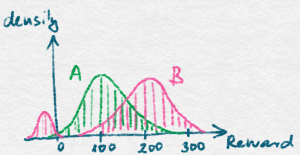
The learner’s goal is to maximize its total reward, $S_n = \sum_{t=1}^n X_t$. Since the $X_t$ are random, $S_n$ is also random and in particular it has a distribution. To illustrate this, the figure on the left shows two possible distributions of the total reward of two different learners, call them $A$ and $B$, but for the same environment. Say, you can choose between learners $A$ and $B$ when running your company whose revenue will be whatever the learner makes. Which one would you choose? One choice is to go with the learner whose total reward distribution has the larger expected value. This will be our choice for most of the class when discussing stochastic environments. Thus, we will prefer algorithms that make the expectation of the total reward gained, symbolically, $\EE{S_n}$, large. This is not the only choice but for now we will stick to it (see some notes on this and other things at the end of this post).

Note that we have not said for which value of $n$ we would like $S_n$ to be large, that is, what horizon do we want to optimize for. We will not go into this issue in detail, but roughly there are two choices. The simplest case is when $n$ is the total number of rounds to be played and is known in advance. Alternatively, if the number of rounds is not known , then one often tries to make $S_n$ large for all $n$ simultaneously. The latter is somewhat delicate, because one can easily believe that there are trade-offs to be made. For now we leave it at that and return to this issue later.

The Bernoulli, Gaussian and uniform distributions are often used as examples for illustrating some specific property of learning in stochastic bandit problems. The Bernoulli distribution (i.e., when the reward is binary valued) is in fact a natural choice – think of applications like maximizing click-through rates in a web-based environment: A click is worth a unit reward, no click means no (zero) reward. If this environment is stationary and stochastic, we get what is called Bernoulli bandits. Similarly, Gaussian bandits means that the payoff distributions are given by Gaussians. Of course, one arm could also have a Bernoulli, another arm could have a Gaussian, the third could have a uniform distribution. More generally, we can have bandits where we only know that the range of rewards is bounded to some interval, or some weaker information, such as the reward distribution has thin tails (i.e., not fat tails).

Decomposing the regret

To formulate the statement about the regret decomposition, let $\mu_k = \int_{-\infty}^{\infty} x P_k(dx)$ be the expected reward gained when action $k$ is chosen (we assume that $P_k$ is such that $\mu_k$ exists and is finite), $\mu^* = \max_k \mu_k$ be the maximal reward and $\Delta_k = \mu^* – \mu_k$. (The range of $k$ here is in $[K]$, i.e., $\mu_k$ and $\Delta_k$ are defined for each $k\in [K]$. To save some typing and to avoid clutter, in the future we will assume that the reader can work out ranges of symbols when we think this can be done in a unique way).

The value of $\Delta_k$ is the expected amount that the learner loses in a single round by choosing action $k$ compared to using an optimal action. This is called the immediate regret of action $k$, and is also known as the action-gap or sub-optimality gap of action $k$. Further, let $T_k(n) = \sum_{t=1}^n \one{A_t = k}$ be the number of times action $k$ was chosen by the learner before the end of round $n$ (including the choice made in round $n$). Here, $\one{\cdot}$ stands for what is called the indicator function, which we use to convert the value of a logical expression (the argument of the indicator function) to either zero (when the argument evaluates to logical false), or one (when the argument evaluates to logical true).

Note that, in general, $T_k(n)$ is also random. This may be surprising if we think about a deterministic learner (a learner which, given the past, decides upon the next action following a specific function, also known as the policy of the learning, without any extra randomization). So why is $T_k(n)$ random in this case? The reason is because for $t>1$, $A_t$ depends on the rewards observed in rounds $1,2,\dots,t-1$, which are random, hence $A_t$ will also inherit their randomness.

The total expected regret of the learner is $R_n = n\mu^* – \EE{\sum_{t=1}^n X_t}$: You should convince yourself that given the knowledge of $(P_1,\dots,P_K)$, a learner could make on expectation $n\mu^*$, but no learner can make more than this in expectation. That is, $n\mu^*$ is the optimal total expected reward in $n$ rounds. Thus, our $R_n$ above is the difference of how much an omniscient decision maker could have made and how much the learner made. At a first sight this definition may sound quite a bit stronger than asking for the difference between of how much an omniscient decision maker who is restricted to choosing the same action in every round could have made, the definition we used in the first post. However, in a stationary stochastic bandit environments there exist optimal omniscient decision makers that would chose the same action in every round. Thus, the two concepts coincide.

The statement mentioned beforehand is as follows:

Lemma (Basic Regret Decomposition Identity): $R_n = \sum_{k=1}^K \Delta_k \EE{ T_k(n) }$.

The lemma simply decomposes the regret in terms of the loss due to using each of the arms. Of course, if $k$ is optimal (i.e., $\mu_k = \mu^*$) then $\Delta_k = 0$. The lemma is useful in that it tells us that to keep the regret small, the learner should try to minimize the weighted sum of expected action-counts, where the weights are the respective action gaps. In particular, a good learner should aim to use an arm with a larger action gap proportionally fewer times.

Proof:
Since $R_n$ is based on summing over rounds, and the right hand side is based on summing over actions, to convert one sum into the other one we introduce indicators. In particular, note that for any fixed $t$ we have $\sum_k \one{A_t=k} = 1$. Hence, $S_n = \sum_t X_t = \sum_t \sum_k X_t \one{A_t=k}$ and thus
\begin{align*}
R_n = n\mu^* – \EE{S_n} = \sum_{k=1}^K \sum_{t=1}^n \EE{(\mu^*-X_t) \one{A_t=k}}.
\end{align*}
Now, knowing $A_t$, the expected reward is $\mu_{A_t}$. Thus we have
\begin{align*}
\EE{ (\mu^*-X_t) \one{A_t=k}\,|\,A_t} = \one{A_t=k} \EE{ \mu^*-X_t\,|\,A_t} = \one{A_t=k} (\mu^*-\mu_{A_t}) = \one{A_t=k} (\mu^*-\mu_{k}).
\end{align*}
Using the definition of $\Delta_k$ and then plugging in into the right-hand side of the previous equation, followed by using the definition of $T_k(n)$ gives the result.
QED.

The proof is as simple as it gets. The technique of using indicators for switching from sums over one variable to another will be used quite a few times, so it is worth remembering. Readers who are happy with the level of detail and feel comfortable with the math can stop reading here. Readers who are asking themselves about what $\EE{X_t\,|\,A_t}$ means, or why various steps of this proof are valid, or even what is the proper definition of all the random variables mentioned, in short, readers who want to develop a rigorous understanding of what went into the above proof, should read on. The rest of the post is not short, but by the end, readers following the discussion should gain a quite solid foundation for the remaining posts. We also promise to provide a somewhat unusual, and hopefully more insightful than usual description of these foundations.

Rigorous foundations

The rigorous foundation to the above, as well as all subsequent results, is based on probability theory, or more precisely, on measure-theoretic probability theory. There are so many textbooks on measure-theoretic probability theory that the list could easily fill a full book itself. At the end, we will list a few of our favourites. Now, measure-theoretic probability theory may sound off-putting to many as something that is overly technical. People who were exposed to measure-theoretic probability often think that it is only needed when dealing with continuous spaces (like the real numbers), and often the attitude is that measure-theoretic probability is only needed for the sake of rigour and is not more than a mere technical annoyance. There is much truth to this (measure-theoretic probability is needed for all these reasons and can be annoying, too), but we claim that measure-theoretic probability can offer much more than rigor if treated properly. This is what we intend to do in the rest of the post.

Probability spaces and random elements

Imagine the following random game: I throw a dice. If the result is four, I throw two more dice. If the result is not four, I throw one dice only. Looking at the newly thrown dice (one or two), I repeat the same, for a total of three rounds. Afterwards, I pay you the sum of the values on the faces of the dice, which becomes the “value” of the game. How much are you willing to pay me to play this game? Games like these were what drove the development of probability theory at the beginning. The game described looks complicated because the number of dice used is itself random.

Now, here is a simple way of dealing with this complication: instead of considering rolling the dice one by one, imagine that sufficiently many (say, more than 7 in this case) dice were rolled before the game has even started (why 7? because in the first round we use one, in the next round at most 2, and in the last round at most 4 dice). Then, with the dice that have been rolled already, the game can be emulated easily. For example, we can order the rolled dice and just take the value of the first dice in the chosen ordering in the first round of the game. If we see a four, we look at the next two dice in the ordering, otherwise we look at the single next dice. Note that this way we completely separate the random acts (rolling the dice) and the game mechanism (which produces values).

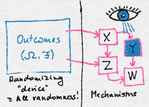
The advantage of this is that we get a simple calculus for the probabilities of all kinds of events. First, the probability of any single outcome of rolling 7 dice, an element of $\Omega \doteq [6]^7$, is simply $1/6^7$ (since all outcomes should be equally probable if the dice are not loaded). The probability of the game payoff taking some value $v$ can then be calculated by calculating the total probability assigned to all those outcomes $\omega\in \Omega$ that, through the complicated game mechanism, would result in the value of $v$. In principle, this is trivial to do thanks to the separation of everything that is probabilistic from the rest. This separation is the essence of probability theory as proposed by Kolmogorov. Or at least the essence of half of probability theory. Here, the set $\Omega$ is called the outcome space, its elements are the outcomes. The figure below illustrates this idea: Random outcomes are generated on the left, while on the right, various mechanisms are used to arrive at values, some of which may be “observed”, some not.

There will be much benefit to being just a bit more formal about how we come up with the value of the game. The major realization is that the process in which the game gets its value is nothing but a function that maps $\Omega$ to the set of natural numbers $\N$. While we view the value of the game as random, this map, call it $X$, is deterministic: The randomness is completely removed from $X$! First point of irony: Functions like $X$, whose domain is the space of outcomes, are called random variables (we will add some extra restriction on these functions soon, but this is a good working definition for now). Furthermore, $X$ is not a variable in a programming language sense and, again, there is nothing random about $X$ itself. The randomness is in the argument that $X$ is acting on, producing “randomly changing” results.

Pick some natural number $v\in \N$. What is the probability of seeing $X=v$? As this was described above, this probability is just $(1/6)^7$ times the cardinality of the set $\set{\omega\in \Omega\,:\,X(\omega)=v}$, which we will denote by $X^{-1}(v)$ and which is called the preimage  (a.k.a. “inverse image”) of $v$ under $X$. More generally, the probability that $X$ takes its value in some set $A\subset \N$ is given by $(1/6)^7$ times the cardinality of $X^{-1}(A) \doteq \set{\omega\in \Omega\,:\,X(\omega)\in A}$ (we have overloaded $X^{-1}$). Here, $X^{-1}(A)$ is also called the preimage of $A$. Note how we always only needed to talk about probabilities assigned to subsets of $\Omega$ regardless of the question asked! It seems that probabilities assigned to subsets are all what one needs for these sort of calculations.

To make this a bit more general, let us introduce a map $\PP$ that assigns probabilities to (certain) subsets of $\Omega$. The intuitive meaning of $\PP$ is now this: Random outcomes are generated in $\Omega$. The probability that an outcome falls into a set $A\subset \Omega$ is $\Prob{A}$. If $A$ is not in the domain of $\PP$, there is no answer to the question of the probability of the outcome falling in $A$. But let’s postpone the discussion of why $\PP$ should be restricted to only certain subsets of $\Omega$ later. In the above example with the dice, $\Prob{ A } = (1/6)^7 |A|$.

With this new notation, the answer to the question of what is the probability of seeing $X$ taking the value of $v$ (or $X=v$) becomes $\Prob{ X^{-1}(v) }$.  To minimize clutter, the more readable notation for this probability is $\Prob{X=v}$. It is important to realize though that the above is exactly the definition of this more familiar symbol sequence! More generally, we also use $\Prob{ \mathrm{predicate}(X,U,V,\dots)} = \Prob{\{\omega \in \Omega : \mathrm{predicate}(X,U,V,\dots) \text{ is true}\}}$ with any predicate, i.e., expression evaluating to true or false, where $X,U,V, \dots$ are functions with domain $\Omega$.

What are the properties that $\PP$ should satisfy? First, we need $\PP(\Omega)=1$ (i.e., it should be defined for $\Omega$ and the probability of an outcome falling into $\Omega$ should be one). Next, for any subset $A\subset \Omega$ for which $\PP$ is defined, $\PP(A)\ge 0$ should hold (no negative probabilities). If $\PP(A^c)$ is also defined where $A^c\doteq \Omega\setminus A$ is the complement of $A$ in $\Omega$, then $\PP(A^c) = 1-\PP(A)$ should hold (negation rule). Finally, if $A,B$ are disjoint (i.e., $A\cap B=\emptyset$) and $\PP(A)$, $\PP(B)$ and $\PP(A\cup B)$ are all defined, then $\PP(A \cup B) = \PP(A) + \PP(B)$ should hold. This is what is called the finite additivity property of $\PP$.

Now, it looks silly to say that $\PP(A^c)$ may not be defined when $\PP(A)$ is defined. Since if $\PP(A^c)$ was not defined, we should just define it as $1-\PP(A)$! Similarly, it is silly if $\PP(A\cup B)$ is not defined for $A,B$ disjoint for which $\PP$ is already defined. Since in this case we should define this value as $\PP(A) + \PP(B)$.

By a logical jump, we will also require the additivity property to hold for countably infinitely many sets: if $\{A_i\}_i$ are disjoint and $\PP(A_i)$ is defined for each $i\in \N$, then $\PP(\cup_i A_i) = \sum_i \PP(A_i)$ should hold. It follows that the set system $\cF$ for which $\PP$ is defined should include $\Omega$, should be closed under complements and countable unions. Such a set system is called a $\sigma$-algebra (sometimes $\sigma$-field). Apart from the requirement of being closed under countable unions (as opposed to finite unions) we see that it is a rather minimal requirement to demand that the set system for which $\PP$ is defined is a $\sigma$-algebra. If $\cF \subseteq 2^\Omega$ is a $\sigma$-algebra and $\PP$ satisfies the above properties then $\PP$ will be called a probability measure. The elements of $\cF$ are called measurable sets: They are measurable in the sense that $\PP$ assigns values to them. The pair $(\Omega,\cF)$ alone is called a measurable space, while the triplet $(\Omega,\cF,\PP)$ is called a probability space. If the condition that $\PP(\Omega)=1$ is lifted $\PP$ is called a measure. If the condition that $\PP(A)\ge 0$ is also lifted then $\PP$ is called a signed measure. We note in passing that both for measures and signed measures it would be unusual to use the symbol $\PP$, which is mostly reserved for probabilities.

Random variables, like $X$, lead to new probability measures. In particular, in our example, $A \mapsto \Prob{ X^{-1}(A) }$ itself is a probability measure defined for all the subsets of $A$ of $\N$ for which $\Prob{ X^{-1}(A) }$ is defined. This probability map is called the distribution induced by $X$ and $\PP$, and is denoted by $\PP_X$. Alternatively, it is also called the pushforward of $\PP$ under $X$. If we want to answer any probabilistic question related to $X$, all we need is just $\PP_X$! It is worth noting that if we keep $X$ but change $\PP$ (e.g, switch to a loaded dice), the distribution of $X$ changes. We will often use arguments that will do exactly this, especially when proving lower bounds about the regret of bandit algorithms.

Now which probability questions related to $X$ can we answer based on a probability map $\PP:\cF \to [0,1]$? The predicates in all these questions take the form $X\in A$ with some $A\subset \N$. Now, to be able to get an answer, we need that $X^{-1}(A)$ is in $\cF$. It can be checked that if we take the set of all the sets of the above form then we get a $\sigma$-algebra. We can also insist that we want to be able to answer questions on the probability of $X\in A$ for any $A\in \cG$ where $\cG$ is some fixed set system (not necessarily a $\sigma$-algebra). If this can be done, we call the $X$ an $\cF/\cG$-measurable map (read: $\cF$-to-$\cG$ measurable). When $\cG$ is obvious from the context, $X$ is often called a measurable map. What is a typical choice for $\cG$? When $X$ is real-valued (being a little more general than in our example) then the typical choice is to let $\cG$ be the set of all open intervals. The reader can verify that if $X$ is $\cF/\cG$-measurable, it is also $\cF/\sigma(\cG)$-measurable where $\sigma(\cG)$ is the smallest $\sigma$-algebra that contains $\cG$. This can be seen to exists and to contain exactly those sets $A$ that are in every $\sigma$-algebra that contains $\cG$. (It is a good practice to prove these statements.) When $\cG$ is the set of open intervals, $\sigma(\cG)$ is the so-called Borel $\sigma$-algebra and $X$ is called a random variable. One can of course consider other range spaces than the set of reals; the ideas still apply. In these cases, instead of random variable, we say that $X$ is a random-element.

You may be wondering why we insist that $\PP$ may not be defined for all subsets of $\Omega$? In fact, in our simple example it would be defined for all subsets of $\Omega$, i.e., $\cF = 2^\Omega$ (and would be in fact given by $\PP(A)=(1/6)^7 | A|$, where $|A|$ is the number of elements of $A$). To understand the advantage of defining $\PP$ only for certain subsets we need to dig a little deeper.

The real reason to use $\sigma$-algebras

Consider this: Let’s say in the game described I tell you the value of $X$. What does the knowledge of $X$ entail? It is clear that knowing the value of $X$ we will also know the value of say $X-1$ or $X^2$ or any nice function of $X$. So anything presented explicitly as “$f(X)$” with nice functions $f$ (e.g., Borel) will be known with certainty when the value of $X$ is known. But what if you have a variable that is not presented explicitly as a function $X$? What can we say about it based on knowing $X$?

For instance, can you tell with certainty the value of the first dice roll $F$? Or can you tell the value of the first dice roll being four, i.e., whether $F=4$? Or the value of $V=\one{F=4,X\ge 7}$, i.e., whether $F=4$ and $X\ge 7$ hold simultaneously? Or the value of $U=\one{F=4,X>24}$? Note that $F,V,U$ are all functions whose domain is $\Omega$. The question whether the value of say, $U$, can be determined with certainty given the value of $X$ is the same as asking whether there exist a function $f$ whose domain is the range of $X$ and whose range is the range of $U$ (binary in this case) such that $U(\omega)=f(X(\omega))$ holds no matter the value of $\omega\in \Omega$. The answer to this specific question is yes: If $X>24$ then $F=4$ because for $F\ne 4$, the maximum value for $X$ is $24$. Thus, $f(x) = \one{x>24}$ will work in this case. In the case of $V$, the answer to the question whether $V$ can be written as a function $X$ is no. Why? What are those random variables that can be determined with certainty given the knowledge of $X$ for some $X$ random variable? As it turns out, there is a very nice answer to this question: Denoting by $\sigma(X)$ the smallest $\sigma$-algebra over $\Omega$ that makes $X$ measurable (this is also called the $\sigma$-algebra generated by $X$), it holds that a random variable $U$ of the same measure space that carries $X$ can be written as a measurable deterministic function of $X$ if and only if $U$ is $\sigma(X)$-measurable. An alternative way of saying this is that $U$ is $\sigma(X)$-measurable if and only if $U$ factorizes into $f$ and $X$ in the sense that $U = f\circ X$ for some $f:\R \to \R$ measurable ($\circ$ stands for the composition of its two arguments). This result is known as the factorization lemma and is one of the core results in probability theory.

The significance of this result cannot be underestimated. The result essentially says that $\sigma(X)$ contains all that there is to know about $X$ in the sense that is suffices to know $\sigma(X)$ if we want to figure out whether some random variable $U$ can be “calculated” based on $X$. In particular, one can forget the values of $X$(!) and still be able to see if $U$ is determined by $X$. One just needs to check whether $\sigma(U) \subset \sigma(X)$. (This may look like a daunting task. The trick to something like this is to work with subsets $\mathcal{E}$ of $\sigma(U)$ such that $\sigma(U)\subset \sigma(\mathcal{E})$.) It also follows that if $X$ and $Y$ generate the same $\sigma$ algebra (i.e., $\sigma(X) = \sigma(Y)$) then if $U$ is determined by $X$ then it is also determined by $Y$ and vice versa. In short, $\sigma(X)$ summarizes all that there is to know about $X$ when it comes to determining what can be computed based on the knowledge of $X$. Without ever explicitly constructing the functions specifying this computation.

Since we see that $\sigma$-algebras are in a way more fundamental than random variables, often we keep the $\sigma$-algebras only, without mentioning any random variables that would have generated them. One can also notice that if $\cG$ and $\cH$ are $\sigma$-algebras and $\cG\subset \cH=\sigma(Y)$ then $\cH$ contains more information in the sense that if a random variable $X$ is $\cG$-measurable, then $X$ is also $\cH$-measurable, hence, $X$ can be written as a deterministic function of $Y$; thus $Y$ (or $\cH$) contains more information than $\cG$.  When we think of $\sigma$-algebras, we are often thinking of all the random variables that are measurable with respect to them.

Now let $X$ be a real-valued random variable and consider taking the restriction of $\PP$ to $\sigma(X)$: $\PP’: \sigma(X) \to [0,1]$, $\PP'(A) = \PP(A)$, $A\in \sigma(X)$. Clearly, $(\Omega,\sigma(X),\PP’)$ is also a probability space. Why should we care? This is a probability space that allows us to answer any question based on knowing $X$ and of all those probability spaces this is the smallest. To break down the first part: Taking any $A\in \sigma(X)$, one can show that there exists $B$ Borel-measurable set such that $A = X^{-1}(B)$. That is, all probabilities for all sets $A$ included in the considered $\sigma$-algebra are probabilities of $X$ being the element of some (Borel-measurable) set $B$. Observe that this probability space has less (not more and potentially much less) detail than the original. Sometimes removing details is what one needs! The process of gradually adding detail is called filtration. More precisely, a filtration is a sequence $(\cF_t)_t$ of $\sigma$-algebras such that $\cF_t \subset \cF_{s}$ for any $t<s$.

Independence and conditional probability

Very often we will want to talk about independent events or independent random variables. Let $(\Omega, \cF, \PP)$ be a probability space and let $X$ and $Y$ be random variables, which by definition means that $X$ and $Y$ are $\cF$-measurable. We say that $X$ and $Y$ are independent if
\begin{align*}
\Prob{X^{-1}(A) \cap Y^{-1}(B)} = \Prob{X^{-1}(A)} \Prob{Y^{-1}(B)}
\end{align*}
for all measurable $A$ and $B$ (note that here $A, B \subseteq \R$ are not elements of $\cF$, but rather of the Borel $\sigma$-algebra that defines the measure space on the reals). A more familiar way of writing the above equation is perhaps
\begin{align*}
\Prob{ X\in A, Y\in B } = \Prob{X\in A} \Prob{Y\in B }\,.
\end{align*}
An alternative way of defining the independence of random variables is in terms of the $\sigma$-algebras they generate. If $\cG$ and $\cH$ are two sub-$\sigma$-algebras of $\cF$, then we say $\cG$ and $\cH$ are independent if $\Prob{A \cap B} = \Prob{A} \Prob{B}$ for all $A \in \cG$ and $B \in \cH$. Then random variables $X$ and $Y$ are independent if and only if the $\sigma$-algebras they generate are independent. An event can be represented by a binary random variable. Let $A, B \in \cF$ be two events, then $A$ and $B$ are independent if $\one{A}$ and $\one{B}$ are independent. If $\Prob{B} > 0$, then we can also define the conditional probability of $A$ given $B$ by
\begin{align*}
\Prob{A|B} = \frac{\Prob{A \cap B}}{\Prob{B}}\,.
\end{align*}
In the special case that $A$ and $B$ are independent this reduces to the statement that $\Prob{A|B} = \Prob{A}$, which reconciles our understanding of independence and conditional probabilities: Intuitively, $A$ and $B$ are independent if knowing whether $B$ happens does not change the probability of whether $A$ happens, and knowing whether $A$ happens does not change the probability of whether $B$ happens.

Note that if $\Prob{B} = 0$, then the above definition of conditional probability cannot be used. While in some cases the quantity $\Prob{A|B}$ cannot have a reasonable definition, often it is still possible to define this meaningfully, as we shall see it in a later section.

Integration and Expectation

Near the beginning of this post we defined the mean of arm $i$ as $\mu_i = \int^\infty_{-\infty} x dP_i(x)$.
This is also called the expectation of $X$ where $X:\Omega \to \R$ is a random variable sampled from $P_i$. We are now in a good position to reconcile this definition with the measure-theoretic view of probability given above. Let $(\Omega, \cF, \PP)$ be a probability space and $X: \Omega \to \R$ be a random variable. We would like to give a definition of the expectation of $X$ (written $\EE{X}$) that does not require us to write a density or to take a discrete sum (of what?). Rather, we want to use only the definitions of $X$ and the probability space $(\Omega, \cF, \PP)$ directly.

We start with the simple case where $X$ can take only finitely many values (eg., $X$ is the outcome of a fair dice). Suppose these values are $\alpha_1,\ldots,\alpha_k$, then the expectation is defined by
\begin{align*}
\EE{X} = \sum_{i=1}^k \Prob{X^{-1}(\{\alpha_i\})} \alpha_i\,.
\end{align*}
Remember that $X$ is measurable, which means that $X^{-1}(\{\alpha_i\})$ is in $\cF$ and the expression above makes sense. For the remainder we aim to generalize this natural definition to the case when $X$ can take on infinitely many values (even uncountably many!).

Rather than use the expectation notation, we prefer to simply define the expectation in terms of the Lebesgue integral and then define the latter in a way that is consistent with the usual definitions of the expectation (and for that matter with Riemann integration).
\begin{align*}
\EE{X} = \int_{\Omega} X d\PP
\end{align*}

Our approach for defining the Lebesgue integral follows a standard path. Recall that $X$ is a measurable function from $\Omega$ to $\R$. We call $X$ a positive simple function if $X$ can be written as
\begin{align*}
X(\omega) = \sum_{i=1}^k \one{\omega \in A_i} \alpha_i\,,
\end{align*}
where $\alpha_i$ is a positive real number for all $i$ and $A_1,\ldots,A_k \in \cF$. (Often, in the definition it is required that the sets $(A_i)_i$ are pairwise disjoint, but this condition is in fact superfluous: Our definition gives the same set of simple functions as the standard one.) Then we define the Lebesgue integral of this kind of simple random variable $X$ by
\begin{align*}
\int_\Omega X d\PP \doteq \sum_{i=1}^k \Prob{A_i} \alpha_i\,.
\end{align*}
This definition corresponds naturally to the discrete version given above by letting $A_i = X^{-1}(\{\alpha_i\})$. We now extend the definition of the Lebesgue integral to positive measurable functions. The idea is to approximate the function using simple functions. Formally, if $X$ is a non-negative random variable (that is, it is a measurable function from $\Omega$ to $[0,\infty)$), then
\begin{align*}
\int_{\Omega} X d\PP \doteq \sup \left\{\int_\Omega h d\PP : h \text{ is simple and } 0 \leq h \leq X\right\}\,,
\end{align*}
where $h \leq X$ if $h(\omega) \leq X(\omega)$ for all $\omega \in \Omega$. Of course this quantity need not exist (the limit hidden by the supremum could tend to infinity). If it does not exist then we say the integral (or expectation) of $X$ is unbounded or does not exist.

Finally, if $X$ is any measurable function (i.e, it may also take negative values), then define $X^+(\omega) = X(\omega) \one{X(\omega) > 0}$ and $X^{-}(\omega) = -X(\omega) \one{X(\omega) < 0}$ so that $X(\omega) = X^+(\omega) – X^-(\omega)$. Then $X^+$ and $X^-$ are non-negative random variables and provided that $\int_{\Omega} X^+ d\PP$ and $\int_\Omega X^- d\PP$ both exist, then we define
\begin{align*}
\int_\Omega X d\PP \doteq \int_\Omega X^+ d\PP – \int_\Omega X^-d\PP\,.
\end{align*}
None of what we have done depends on $\PP$ being a probability measure (that is $\Prob{A} \geq 0$ and $\Prob{\Omega} = 1$). The definitions all hold more generally for any measure and in particular, if $\Omega = \R$ is the real line and $\cF$ is the Lebesgue $\sigma$-algebra (defined in the notes below) and the measure is the so called Lebesgue measure $\lambda$, which is the unique measure such that $\lambda((a,b)) = b-a$ for any $a \leq b$. In this scenario, if $f:\R \to \R$ is a measurable function, then we can write the Lebesgue integral of $f$ with respect to the Lebesgue measure as
\begin{align*}
\int_{\R} f \,d\lambda\,.
\end{align*}
Perhaps unsurprisingly this almost always coincides with the improper Riemann integral of $f$, which is normally written as $\int^\infty_{-\infty} f(x) dx$. Precisely, if $|f|$ is both Lebesgue integrable and Riemann integrable, then the integrals are equal. There do, however, exist functions that are Riemann integrable and not Lebesgue integrable, and also the other way around (although examples of the former are more unusual than the latter).

Having defined the expectation of a random variable in terms of the Lebesgue integral, one might ask about the properties of the expectation. By far the most important property is its linearity. Let $X_i$ be a (possibly infinite) set of random variables on the same probability space and assume that $\EE{X_i}$ exists for all $i$ and furthermore that $X = \sum_i X_i$ and $\EE{X}$ also exist. Then
\begin{align*}
\EE{X} = \sum_i \EE{X_i}\,.
\end{align*}
This property, “swapping the order of $\E$ and $\sum_i$”, is the source of much magic in probability theory because it holds even if $X_i$ are not independent. This means that (unlike probabilities) we can very often decouple the expectations of dependent random variables, which often proves extremely useful. We will not prove this statement here, but as usual suggest the reader do so for themselves. The other requirement for linearity is that if $c \in \R$ is a constant, then $\EE{c X} = c \EE{X}$, which is also true and rather easy to prove. Note that if $X$ and $Y$ are independent, then one can show that $\EE{X Y} = \EE{X} \EE{Y}$, but this is not true in general for dependent random variables (try to come up with a simple example demonstrating this).

Conditional expectation

Besides the expectation, we will also need conditional expectation, which allows us to talk about the expectation of a random variable given the value of another random variable. To illustrate with an example, let $\Omega = [6]$ (the outcomes of a dice) and $\cF = 2^\Omega$ and $\PP$ is the uniform measure on $\Omega$ so that $\Prob{A} = |A|/6$ for each $A \in \cF$. Define two random variables $X,Y$, with $Y(\omega) = \one{\omega > 3}$ and $X(\omega) = \omega$ and suppose that only $Y$ is observed. Given a specific value of $Y$ (say, $Y = 1$), what can be said about the expectation of $X$? Arguing intuitively, we might notice that $Y=1$ means that the unobserved $X$ must be either $4$, $5$ or $6$, and that each of these outcomes is equally likely and so the expectation of $X$ given that $Y=1$ should be $(4+5+6)/3 = 5$. Similarly, the expectation of $X$ given $Y=0$ should be $(1+2+3)/3=2$. If we want a concise summary, we can just write that “the expectation of $X$ given $Y$” is $5Y + 2(1-Y)$. Notice how this is a random variable itself! The notation for the expectation of $X$ conditioned on the knowledge of $Y$ is $\EE{X|Y}$. Thus, in the above example, $\EE{X|Y} = 5Y + 2(1-Y)$. Similar question: Say, $X$ is Bernoulli with parameter $P$, where $P$ is a uniformly distributed random variable on $[0,1]$. Since the expectation of a Bernoulli random variable with fixed (nonrandom) parameter $q$ is $q$, intuitively, knowing $P$, we should get that the expectation of $X$, given $P$ is just $P$: $\EE{X|P}=P$. More generally, for any $X,Y$, $\EE{X|Y}$ should be a function of $Y$. In other words, $\EE{X|Y}$ should be $\sigma(Y)$ measurable! Also, if we replace $Y$ with $Z$ such that $\sigma(Z) = \sigma(Y)$, should $\EE{X|Z}$ be different than $\EE{X|Y}$? Take for example, $Q=1-P$ and let $X$ be Bernoulli with parameter $P$ still. We have $\EE{X|P} = P$. What is $\EE{X|Q}$? Again, intuitively, $\EE{X|Q} = 1-Q$ should hold (if $Q=1$, $P=0$, the expected value of $X$ with parameter zero is zero, etc.) But $1-Q= P$, hence $\EE{X|Q}=P$. At the end, what matters is not what specific random variable we are conditioning on, but the knowledge contained in that random variable, which is encoded by the $\sigma$-algebra it generates. So, how should we construct, or define conditional expectations to align them with the above intuitions, and to be rigorous (even in case like the above when for any particular $p\in [0,1]$, $\Prob{P=p}=0$!).

This is done as follows: Let $(\Omega, \cF, \PP)$ be a probability space and $X: \Omega \to \R$ be random variable and $\cH$ be a sub-$\sigma$-algebra of $\cF$. The conditional expectation of $X$ given $\cH$ is a $\cH$-measurable random variable that is denoted by $\E[X|\cH]$ and defined to be any $\cH$-measurable random variable such that for all $H \in \cH$,
\begin{align*}
\int_H \E[X|\cH] d\PP = \int_H X d\PP\,.
\end{align*}
Given a $\cF$-measurable random variable $Y$, the conditional expectation of $X$ given $Y$ is $\EE{X|Y} = \EE{X|\sigma(Y)}$. Again, at the risk of being a little overly verbose, what is the meaning of all this? Returning to the dice example above we see that $\EE{X|Y} = \EE{X|\sigma(Y)}$ and $\sigma(Y) = \{\{1,2,3\}, \{4,5,6\}\, \emptyset, \Omega\}$. Now the condition that $\E[X|\cH]$ is $\cH$-measurable can only be satisfied if $\E[X|\cH](\omega)$ is constant on $\{1,2,3\}$ and $\{4,5,6\}$ and then the display equation above immediately implies that
\begin{align*}
\EE{X|\cH}(\omega) = \begin{cases}
2, & \text{if } \omega \in \{1,2,3\}\,; \\
5, & \text{if } \omega \in \{4,5,6\}\,.
\end{cases}
\end{align*}
Finally, we want to emphasize that the definition of conditional expectation given above is not constructive. Even more off-putting is that $\E[X|\cH]$ is not even uniquely defined, although it is uniquely defined up to a set of measure zero that can safely be disregarded in calculations. A related notation that will be useful is as follows: If $X=Y$ up to a zero measure set according to $\PP$, i.e., the “exceptional set” $\{\omega\in \Omega\,: X(\omega) \ne Y(\omega)\}$ has a zero $\PP$-measure, then we write $X=Y$ $\PP$-almost surely, or, in abbreviated form $X=Y$ ($\PP$-a.s.). Sometimes this is expressed in the literature by “$X=Y$ with probability one”, which agrees with $\Prob{X\ne Y}=0$.

Let us summarize some important properties of conditional expectations (which follow from the definition directly):

Theorem (Properties of Conditional Expectations): Let $(\Omega,\cF,\PP)$ be a probability space, $\cG\subset \cF$ a sub-$\sigma$-algebra of $\cF$, $X,Y$ random variables on $(\Omega,\cF,\PP)$.

• $\EE{X|\cG} \ge 0$ if $X\ge 0$ ($\PP$-a.s.);
• $\EE{1|\cG} = 1$ ($\PP$-a.s.);
• $\EE{ X+Y|\cG } = \EE{ X|\cG } + \EE{ Y|\cG }$ ($\PP$-a.s.), assuming the expression on the right-hand side is defined;
• $\EE{ XY|\cG } = Y \EE{X|\cG}$ if $\EE{XY}$ exists and $Y$ is $\cG$-measurable;
• if $\cG_1\subset \cG_2 \subset \cF$ then ($\PP$-a.s.) $\EE{ X|\cG_1 } = \EE{ \EE{ X|\cG_2} | \cG_1 }$;
• if $\cG$ and $\cF$ are independent then ($\PP$-a.s.) $\EE{X|\cG} = \EE{X}$. In particular, if $\cG = \{\emptyset,\Omega\}$ is the trivial $\sigma$-algebra then $\EE{ X|\cG } = \EE X$ ($\PP$-a.s.).

 

Notes and departing thoughts

This was a long post. If you are still with us, good. Here are some extra thoughts. At the end of this section the notes return to the bandit problem that we started with.

Note 1: It is not obvious why the expected value is a good summary of the reward distribution. Decision makers who base their decisions on expected values are called risk-neutral. In the example shown on the figure above, a risk-averse decision maker may actually prefer the distribution labeled as $A$ because occasionally distribution $B$ may incur a very small (even negative) reward. Risk-seeking decision makers, if they exist at all, would prefer distributions with occasional large rewards to distributions that give mediocre rewards only. There is a formal theory of what makes a decision maker rational (a decision maker in a nutshell is rational if he/she does not contradict himself/herself). Rational decision makers compare stochastic alternatives based on the alternatives’ expected utilities, according to a theorem of von Neumann and Morgenstern. Humans are known to be not doing this, i.e., they are irrational. No surprise here.

Note 2: Note that in our toy example instead of $\Omega=[6]^7$, we could have chosen $\Omega = [6]^8$ (considering rolling eight dice instead of 7, one dice never used). There are many other possibilities. We can consider coin flips instead of dice rolls (think about how this could be done). To make this easy, we could use weighted coins (e.g, a coin lands on its head with probability 1/6), but we don’t actually need weighted coins (this may be a little tricky to see). The main point is that there are many ways to emulate one randomization device by using another. The difference between these is the set $\Omega$. What makes a choice of $\Omega$ viable is if we can emulate the game mechanism on the top of $\Omega$ so that in the end the probability of seeing any particular value remains the same. In other words, the choice of $\Omega$ is far from unique. The same is true for the way we calculate the value of the game! For example, the dice could be reordered, if we stay with the first construction. The biggest irony in all probability theory is that we first make a big fuss about introducing $\Omega$ and then it turns out that the actual construction of $\Omega$ does not matter.

Note 3: The Lebesgue $\sigma$-algebra is obtained as the completion of the Borel $\sigma$-algebra with the following process: Take the null-sets in the Borel $\sigma$-algebra, i.e., the sets which have zero Lebesgue measure (one first constructs the Lebesgue measure for the Borel sets). Add all these to the Borel sets and then close the resulting set to make it again a $\sigma$-algebra. The resulting set is the Lebesgue $\sigma$-algebra and the Lebesgue measure is then extended to this set. With the same process, we can complete any $\sigma$-algebra with respect to some chosen measure. Incomplete $\sigma$-algebras are annoying to work with as one can meet sets that have a zero measure superset but whose measure is not defined.

Note 4: We did not talk about this, but there is a whole lot to say about why the sum, or the product of random variables are also random variables, or why $\inf_n X_n$, $\sup_n X_n$, $\liminf_n X_n$, $\limsup_n X_n$ are measurable when $X_n$ are, just to list a few things. For studying sums, products, etc, the key point is to show first that the composition of measurable maps is also a measurable map and that continuous maps are measurable, and then apply these results. For $\limsup_n X_n$, just rewrite it as $\lim_{m\to\infty} \sup_{n\ge m} X_n$, note that $\sup_{n\ge m} X_n$ is decreasing (we take suprema of smaller sets as $m$ increases), hence $\limsup_n X_n = \inf_m \sup_{n\ge m} X_n$, reducing the question to studying $\inf_n X_n$ and $\sup_n X_n$. Finally, for $\inf_n X_n$ note that it suffices if $\{\omega\,:\,\inf_n X_n \ge t\}$ is measurable any $t$ real. Now, $\inf_n X_n \ge t$ if and only if $X_n\ge t$ for all $n$. Hence, $\{\omega\,:\,\inf_n X_n \ge t\} = \cap_n \{\omega\,:\,X_n \ge t\}$, which is a countable intersection of measurable sets, hence measurable.

Note 5: The factorization lemma (attributed to Joseph L. Doob, the developer of the theory of martingales and author of the classic book “Stochastic Processes”) sneakily uses the properties of real numbers (think about why). So what we said about $\sigma$-algebras containing all information is mostly true. There are extensions, e.g., to Polish spaces, essentially covering all the interesting cases. In some sense the key is that the $\sigma$-algebra of the image space of the variable whose factorization we are seeking should be rich enough.

Note 6: We did not talk about basic results, like Lebesgue’s dominated, monotone convergence theorems, or Fatou’s lemma, or Jensen’s inequality. Of these, we will definitely use the last.

Note 7: The Radon-Nykodim derivative is what helps one to define conditional expectations with the required properties.

Save

Save

Note 8: With the help of conditional expectations, the protocol in the bandit problem requires that for any Borel set $U$,
\begin{align}
\label{eq:condprobconstraint}
\Prob{X_t \in U|A_1,X_1,\dots,A_{t-1},X_{t-1},A_t} = P_{A_t}(U)\,.
\end{align}
Now, you should go back and see whether you can prove the lemma based on the information in this post.

Note 9: In full formality, the lemma, and many of the subsequent results would read as follows: For all probability spaces $(\Omega,\cF,\PP)$ and for any infinite sequence of random variables $(A_1,X_1,\dots)$ such that for all $t\ge 1$, $A_t$ is $\sigma(A_1,X_1,\dots,A_{t-1},X_{t-1})$-measurable, and $X_t$ satisfies $\eqref{eq:condprobconstraint}$ for any Borel set $U$, it holds that $\dots$. Think about this: There are many choices for all these things. The statement guarantees universality: No matter how we chooses these things, the statement will hold. This is how probability spaces are there, but they are never mentioned. Why did we just say that $A_t$ is $\sigma(A_1,X_1,\dots,A_{t-1},X_{t-1})$-measurable? What is the meaning of this?

Note 10: If we want to account for randomized algorithms, all that we have to do is to replace in $\eqref{eq:condprobconstraint}$ $\sigma(A_1,X_1,\dots,A_{t-1},X_{t-1},A_t)$ ($t\ge 1$) with an increasing sequence of $\sigma$-algebras $(\cF_t)_{t\ge 1}$ such that $A_t$ is $\cF_t$-measurable, and $X_t$ is $\cF_{t+1}$-measurable. Why?

Note 11: But can we even construct a probability space $(\Omega,\cF,\PP)$ that can hold the infinitely many random variables $(X_1,A_1,\dots)$ that we need for our protocol with the required properties? There is a theorem by Ionescu Tulcea, which assures that this is the case. Kolmogorov’s extension theorem is another well-known result of this type, but for our purposes the theorem of Ionescu Tulcea is more suitable.

Note 12: We also wanted to add a few words about regular conditional probability measures, but the post is already too long. Maybe another time.

We mentioned that we will give some references. Here is at least one: In terms of its notation, David Pollard’s “A measure theoretic guide to probability” is perhaps somewhat unusual (it follows de Finetti’s notation, where $\PP$ is eliminated as redundant and gets replaced by $\mathbb E$ and sets stand for their indicator functions, etc.). This may put off some people. It should not! First, the notation is in fact quite convenient (if unusual). But the main reason I recommend it is because it is very carefully written and explains much more about the why and how than many other books. Our text was also inspired by this book.

Save

Save

Save

Save