With most of the background material out of the way, we are almost ready to start designing algorithms for finite-armed stochastic bandits and analyzing their properties, and especially the regret. The last thing we need is an introduction to concentration of measure. As we have already seen, the regret measures the difference between the rewards you would expect to obtain if you choose the optimal action in every round, and the rewards you actually expect to see by using your policy. Of course the optimal action is the one with the largest mean and the mean payoffs of the actions are not known from the beginning but must be learned from data. We now ask how long it takes to learn about the mean reward of an action.
Suppose that $X_1,X_2,\ldots,X_n$ is a sequence of independent and identically distributed random variables (see the notes of the last post to see how one sets this up formally). Let $X$ be another random variable sharing the common distribution of the $X_i$s. Assume that the mean $\mu = \EE{X}$ exists (by construction, $\mu = \EE{X_i}$ for $i\in [n]$). Having observed $X_1,X_2,\ldots,X_n$ we would like to define an estimator of the common mean $\mu$ of the $X_i$ random variables. Of course the natural choice to estimate $\mu$ is to use the average of the observations, also known as the sample mean or empirical mean:
\begin{align*}
\hat \mu \doteq \frac{1}{n} \sum_{i=1}^n X_i\,.
\end{align*}
Note that $\hat \mu$ is itself a random variable. The question is how far from $\mu$ do we expect $\hat \mu$ to be? First, by the linearity of $\E$, we can notice that $\EE{\hat \mu} = \mu$. A simple measure of the spread of the distribution of a random variable $Z$ is its variance, defined by $\VV{Z} \doteq \EE{ (Z-\EE{Z})^2 }$. Applying this to the sample mean $\hat \mu$, a quick calculation shows that $\VV{\hat \mu} = \sigma^2 / n$ where $\sigma^2$ is the variance of $X$. From this, we get
\begin{align}\label{eq:iidvarbound}
\EE{(\hat \mu – \mu)^2} = \frac{\sigma^2}{n}\,,
\end{align}
which means that we expect the squared distance between $\mu$ and $\hat \mu$ to shrink as $n$ grows large at rate $1/n$ and scale linearly with the variance of $X$ (so larger variance means larger expected squared difference). While the expected squared error is important, it does not tell us very much about the distribution of the error. To do this we usually analyze the probability that $\hat \mu$ overestimates or underestimates $\mu$ by more than some value $\epsilon > 0$. Precisely, how do the following quantities depend on $\epsilon$?
\begin{align*}
\Prob{\hat \mu \geq \mu + \epsilon} \quad\text{ and }\quad \Prob{\hat \mu \leq \mu – \epsilon}
\end{align*}
The quantities above (as a function of $\epsilon$) are often called the tail probabilities of $\hat \mu – \mu$, see the figure below. In particular, the first is called an upper tail probability, while the second the lower tail probability. Analogously, the probability $\Prob{|\hat \mu -\mu|\geq \epsilon}$ is called a two-sided tail probability.
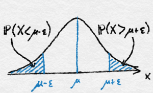
The tails are where $X$ takes on large or small values.
By combining $\eqref{eq:iidvarbound}$ with Chebyschev’s inequality we can bound the two-sided tail directly by
\begin{align*}
\Prob{|\hat \mu – \mu| \geq \epsilon} \leq \frac{\sigma^2}{n \epsilon^2}\,.
\end{align*}
This result is nice because it was so easily bought and relied on no assumptions other than the existence of the mean and variance. The downside is that in many cases the inequality is extremely loose and that huge improvement is possible if the distribution of $X$ is itself “nicer”. In particular, by assuming that higher moments of $X$ exist, Chebyshev’s inequality can be greatly improved, by applying Markov’s inequality to $|\hat \mu – \mu|^k$ with the positive integer $k$ to be chosen so that the resulting bound is optimized. This is a bit cumbersome and while this method is essentially as effective as the one we present below (which can be thought of as the continuous analog of choosing $k$), the method we present looks more elegant.
To calibrate our expectations on what gains to expect over Chebyshev’s inequality, let us first discuss the central limit theorem. Let $S_n = \sum_{t=1}^n (X_t – \mu)$. Informally, the central limit theorem (CLT) says that $S_n / \sqrt{n}$ is approximately distributed like a Gaussian with mean zero and variance $\sigma^2$. This would suggest that
\begin{align*}
\Prob{\hat \mu \geq \mu + \epsilon}
&= \Prob{S_n / \sqrt{n} \geq \epsilon \sqrt{n}} \\
&\approx \int^\infty_{\epsilon \sqrt{n}} \frac{1}{\sqrt{2\pi \sigma^2}} \exp\left(-\frac{x^2}{2\sigma^2}\right) dx\,.
\end{align*}
The integral has no closed form solution, but is easy to bound:
\begin{align*}
\int^\infty_{\epsilon \sqrt{n}} \frac{1}{\sqrt{2\pi \sigma^2}} \exp\left(-\frac{x^2}{2\sigma^2}\right) dx
&\leq \frac{1}{\epsilon \sqrt{2n\pi \sigma^2}} \int^\infty_{\epsilon \sqrt{n}} x \exp\left(-\frac{x^2}{2\sigma^2}\right) dx \\
&= \sqrt{\frac{\sigma^2}{2\pi n \epsilon^2}} \exp\left(-\frac{n\epsilon^2}{2\sigma^2}\right)\,.
\end{align*}
This quantity is almost always much smaller than what we obtained using Chebyschev’s inequality. In particular, it decays slightly faster than the negative exponential of $n \epsilon^2/\sigma^2$. Thus, the measure defined by the mean $\hat \mu$ rapidly concentrates around its mean. Unfortunately, since the central limit theorem is asymptotic, we cannot use it to study the regret when the number of rounds is a fixed finite number. Despite the folk-rule that $n = 30$ is sufficient for the Gaussian approximation brought by CLT to be reasonable, this is simply not true. One well known example is provided by Bernoulli variables with parameter $p \approx 1/n$, in which case the distribution of the average is known to be much better approximated by the Poisson distribution with parameter one, which is nowhere near similar to the Gaussian distribution. Furthermore, it is not hard to believe that the asymptotic behavior of an algorithm is a poor predictor of its finite time behavior, hence it is vital to take a closer look at measure concentration and prove a “version” of the CLT that is true even for small values of $n$.
To prove our measure concentration results, it is necessary to make some assumptions. In order to move rapidly towards bandits we start with a straightforward and relatively fundamental assumption on the distribution of $X$, known as the subgaussian assumption.
Definition (subgaussianity) A random variable $X$ is $\sigma^2$-subgaussian if for all $\lambda \in \R$ it holds that $\EE{\exp(\lambda X)} \leq \exp\left(\lambda^2 \sigma^2 / 2\right)$
The function $M_X(\lambda) = \EE{\exp(\lambda X)}$ is called the moment generating function of $X$ and appears often in probability theory. Note that $M_X(\lambda)$ need not exist for all random variables and the definition of a subgaussian random variable is implicitly assuming this existence.
Lemma: Suppose that $X$ is $\sigma^2$-subgaussian and $X_1$ and $X_2$ are independent and $\sigma^2_1$ and $\sigma^2_2$-subgaussian respectively, then:
- $\E[X] = 0$ and $\VV{X} \leq \sigma^2$.
- $cX$ is $c^2\sigma^2$-subgaussian for all $c \in \R$.
- $X_1 + X_2$ is $(\sigma^2_1 + \sigma^2_2)$-subgaussian.
The proof of the lemma is left as an exercise (hint: Taylor series). Note that in the lack of independence $X_1+X_2$ is $(\sigma_1+\sigma_2)^2$; independence improves this to $\sigma_1^2 + \sigma_2^2$. We are now ready for our key concentration inequality.
Theorem: If $X$ is $\sigma^2$-subgaussian, then $\Prob{X \geq \epsilon} \leq \exp\left(-\frac{\epsilon^2}{2\sigma^2}\right)$.
Proof
We take a generic approach called Chernoff’s method. Let $\lambda > 0$ be some constant to be tuned later. Then
\begin{align*}
\Prob{X \geq \epsilon}
&= \Prob{\exp\left(\lambda X\right) \geq \exp\left(\lambda \epsilon\right)} \\
\tag{Markov’s inequality} &\leq \EE{\exp\left(\lambda X\right)} \exp\left(-\lambda \epsilon\right) \\
\tag{Def. of subgaussianity} &\leq \exp\left(\frac{\lambda^2 \sigma^2}{2} – \lambda \epsilon\right)\,.
\end{align*}
Now $\lambda$ was any positive constant, and in particular may be chosen to minimize the bound above, which is achieved by $\lambda = \epsilon / \sigma^2$.
QED
Combining the previous theorem and lemma leads to a very straightforward analysis of the tails of $\hat \mu – \mu$ under the assumption that $X_i – \mu$ are $\sigma^2$-subgaussian. Since $X_i$ are assumed to be independent, by the lemma it holds that $\hat \mu – \mu = \sum_{i=1}^n (X_i – \mu) / n$ is $\sigma^2/n$-subgaussian. Then by the theorem leads to a bound on the tails of $\hat \mu$:
Corollary (Hoeffding’s bound): Assume that $X_i-\mu$ are independent, $\sigma^2$-subgaussian random variables. Then, their average $\hat\mu$ satisfies
\begin{align*}
\Prob{\hat \mu \geq \mu + \epsilon} \leq \exp\left(-\frac{n\epsilon^2}{2\sigma^2}\right)
\quad \text{ and } \quad \Prob{\hat \mu \leq \mu -\epsilon} \leq \exp\left(-\frac{n\epsilon^2}{2\sigma^2}\right)\,.
\end{align*}
By the inequality $\exp(-x) \leq 1/(ex)$, which holds for all $x \geq 0$ we can see that except for a very small $\epsilon$ the above inequality is strictly stronger than what we obtained via Chebyshev’s inequality and exponentially smaller (tighter) if $n \epsilon^2$ is large relative to $\sigma^2$.
Before we finally return to bandits, one might be wondering what variables are subgaussian? We give two fundamental examples. The first is if $X$ is Gaussian with zero mean and variance $\sigma^2$, then $X$ is $\sigma^2$-subgaussian. The second is bounded zero mean random variables. If $\EE{X}=0$ and $|X| \leq B$ almost surely for some $B \geq 0$, then $X$ is $B^2$-subgaussian. A special case is when $X$ is a shifted Bernoulli with $\Prob{X = 1 – p} = p$ and $\Prob{X = -p} = 1-p$. In this case it also holds that $X$ is $1/4$-subgaussian.
We will be returning to measure concentration many times throughout the course, and note here that it is a very interesting (and still active) topic of research. What we have done and seen is only the very tip of the iceberg, but it is enough for now.
The explore-then-commit strategy
With the background on concentration out of the way we are ready to present the first strategy of the course. The approach, which is to try each action/arm a fixed number of times (exploring) and subsequently choose the arm that had the largest payoff (exploiting), is possibly the simplest approach there is and it is certainly one of the first that come to mind immediately after learning about the definition of a bandit problem. In what follows we assume the noise for all rewards is $1$-subgaussian, by which we mean that $X_t – \E[X_t]$ is $1$-subgaussian for all $t$.
Remark: We assume $1$-subgaussian noise for convenience, in order to avoid endlessly writing $\sigma^2$. All results hold for other values of $\sigma^2$ just by scaling. The important point is that all the algorithms that follow rely on the knowledge of $\sigma^2$. More about this in the notes at the end of the post.
The explore-then-commit strategy is characterized by a natural number $m$, which is the number of times each arm will be explored before committing. Thus the algorithm will explore for $mK$ rounds before choosing a single action for the remaining $n – mK$ rounds. We can write this strategy formally as
\begin{align*}
A_t = \begin{cases}
i\,, & \text{if } (t \operatorname{mod} K)+1 = i \text{ and } t \leq mK\,; \\
\argmax_i \hat \mu_i(mK)\,, & t > mK\,,
\end{cases}
\end{align*}
where ties in the argmax will be broken in a fixed arbitrary way and $\hat \mu_i(t)$ is the average pay-off for arm $i$ up to round $t$:
\begin{align*}
\hat \mu_i(t) = \frac{1}{T_i(t)} \sum_{s=1}^t \one{A_s = i} X_s\,.
\end{align*}
where recall that $T_i(t) = \sum_{s=1}^t \one{A_s=i}$ is the number of times action $i$ was chosen up to the end of round $t$. In the ETC strategy, $T_i(t)$ is deterministic for $t \leq mK$ and $\hat \mu_i(t)$ is never used for $t > mK$. However, in other strategies (that also use $\hat\mu_i(t)$) $T_i(t)$ could be genuinely random (i.e., not concentrated on a single deterministic quantity like here). In those cases, the concentration analysis of $\hat \mu_i(t)$ will need to take the randomness of $T_i(t)$ properly into account. In the case of ETC, the concentration analysis of $\hat \mu_i(t)$ is simple: $\hat \mu_i(t)$ is the average of $m$ independent, identically distributed random variables, hence the corollary above applies immediately.
The formal definition of the explore-then-commit strategy leads rather immediately to the analysis of its regret. First, recall from the previous post that the regret can be written as
\begin{align*}
R_n = \sum_{t=1}^n \EE{\Delta_{A_t}}\,.
\end{align*}
Now in the first $mK$ rounds the strategy given above is completely deterministic, choosing each action exactly $m$ times. Subsequently it chooses a single action that gave the largest average payoff during exploring. Therefore, by splitting the sum we have
\begin{align*}
R_n = m \sum_{i=1}^K \Delta_i + (n-mK) \sum_{i=1}^K \Delta_i \Prob{i = \argmax_j \hat \mu_j(mK)}\,,
\end{align*}
where again we assume that ties in the argmax are broken in a fixed specific way. Now we need to bound the probability in the second term above. Assume without loss of generality that the optimal arm is $i = 1$ so that $\mu_1 = \mu^* = \max_i \mu_i$ (though the learner does not know this). Then,
\begin{align*}
\Prob{i = \argmax_j \hat \mu_j(mK)}
&\leq \Prob{\hat \mu_i(mK) – \hat \mu_1(mK) \geq 0} \\
&= \Prob{\hat \mu_i(mK) – \mu_i – \hat \mu_1(mK) + \mu_1 \geq \Delta_i}\,.
\end{align*}
The next step is to check that $\hat \mu_i(mK) – \mu_i – \hat \mu_1(mK) + \mu_1$ is $2/m$-subgaussian, which by the properties of subgaussian random variables follows from the definitions of $\hat \mu_i$ and the algorithm. Therefore, by the theorem in the previous section (also by our observation above) we have
\begin{align*}
\Prob{\hat \mu_i(mK) – \mu_i – \hat \mu_1(mK) + \mu_1 \geq \Delta_i} \leq \exp\left(-\frac{m \Delta_i^2}{4}\right)
\end{align*}
and by straightforward substitution we obtain
\begin{align}
\label{eq:etcregretbound}
R_n \leq m \sum_{i=1}^K \Delta_i + (n – mK) \sum_{i=1}^K \Delta_i \exp\left(-\frac{m\Delta_i^2}{4}\right)\,.
\end{align}
To summarize:
Theorem (Regret of ETC): Assume that the noise of the reward of each arm in a $K$-armed stochastic bandit problem is $1$-subgaussian. Then, after $n\ge mK$ rounds, the expected regret $R_n$ of ETC which explores each arm exactly $m$ times before committing is bounded as shown in $\eqref{eq:etcregretbound}$.
Although we will discuss many disadvantages of this algorithm, the above bound cleanly illustrates the fundamental challenge faced by the learner, which is the trade-off between exploration and exploitation. If $m$ is large, then the strategy explores very often and the first term will be relatively larger. On the other hand, if $m$ is small, then the probability that the algorithm commits to the wrong arm will grow and the second term becomes large. The big question is how to choose $m$? If we limit ourselves to $K = 2$, then $\Delta_1 = 0$ and by using $\Delta = \Delta_2$ the above display simplifies to
\begin{align*}
R_n \leq m \Delta + (n – 2m) \Delta \exp\left(-\frac{m\Delta^2}{4}\right)
\leq m\Delta + n \Delta \exp\left(-\frac{m\Delta^2}{4}\right)\,.
\end{align*}
Provided that $n$ is reasonably large this quantity is minimized (up to a possible rounding error) by
\begin{align*}
m = \ceil{\frac{4}{\Delta^2} \log\left(\frac{n \Delta^2}{4}\right)}
\end{align*}
and for this choice the regret is bounded by
\begin{align}
\label{eq:regret_g}
R_n \leq \Delta + \frac{4}{\Delta} \left(1 + \log\left(\frac{n \Delta^2}{4}\right)\right)\,.
\end{align}
As we will eventually see, this result is not far from being optimal, but there is one big caveat. The choice of $m$ given above (which defines the strategy) depends on $\Delta$ and $n$. While sometimes it might be reasonable that the horizon is known in advance, it is practically never the case that the sub-optimality gaps are known. So is there a reasonable way to choose $m$ that does not depend on the unknown gap? This is a useful exercise, but it turns out that one can choose an $m$ that depends on $n$, but not the gap in such a way that the regret satisfies $R_n = O(n^{2/3})$ and that you cannot do better than this using an explore-then-commit strategy. At the price of killing the suspense, there are other algorithms that do not even need to know $n$ that can improve this rate significantly to $O(n^{1/2})$.
Setting this issue aside for a moment and returning to the regret guarantee above, we notice that $\Delta$ appears in the denominator of the regret bound, which means that as $\Delta$ becomes very small the regret grows unboundedly. Is that reasonable and why is it happening? By the definition of the regret, when $K = 2$ we have a very trivial bound that follows because $\sum_{i=1}^K \E[T_i(n)] = n$, giving rise to
\begin{align*}
R_n = \sum_{i=1}^2 \Delta_i \E[T_i(n)] = \Delta \E[T_2(n)] \leq n\Delta\,.
\end{align*}
This means that if $\Delta$ is very small, then the regret must also be very small because even choosing the suboptimal arm leads to only minimal pain. The reason the regret guarantee above does not capture this is because we assumed that $n$ was very large when solving for $m$, but for small $n$ it is not possible to choose $m$ large enough that the best arm can actually be identified at all, and at this point the best reasonable bound on the regret is $O(n\Delta)$. To summarize, in order to get a bound on the regret that makes sense we can take the minimum of the bound proven in \eqref{eq:regret_g} and $n\Delta$:
\begin{align*}
R_n \leq \min\left\{n\Delta,\, \Delta + \frac{4}{\Delta}\left(1 + \log\left(\frac{n\Delta^2}{4}\right)\right)\right\}\,.
\end{align*}
We leave it as an exercise to the reader to check that provided $\Delta \leq \sqrt{n}$, then $R_n = O(\sqrt{n})$. Bounds of this nature are usually called worst-case or problem-free or problem independent. The reason is that the regret depends only on the distributional assumption, but not on the means. In contrast, bounds that depend on the sub-optimality gaps are called problem/distribution dependent.
Notes
Note 1: The Berry-Esseen theorem quantifies the speed of convergence in the CLT. It essentially says that the distance between the Gaussian and the actual distribution decays at a rate of $1/\sqrt{n}$ under some mild assumptions. This is known to be tight for the class of probability distributions that appear in the Berry-Esseen result. However, this is a poor result when the tail probabilities themselves are much smaller than $1/\sqrt{n}$. Hence, the need for alternate results.
Note 2: The Explore-then-Commit strategy is also known as the “Explore-then-Exploit” strategy. A similar idea is to “force” a certain amount of exploration. Policies that are based on forced exploration ensure that each arm is explored (chosen) sufficiently often. The exploration may happen upfront like in ETC, or spread out in time. In fact, the limitation of ETC that it needs to know $n$ even to achieve the $O(n^{2/3})$ regret can be addressed by this (e.g., using the so-called “doubling trick”, where the same strategy that assumes a fixed horizon is used on horizons of length that increase at some rate, e.g., they could double). The $\epsilon$-greedy strategy chooses a random action with probability $\epsilon$ in every round, and otherwise chooses the action with the highest mean. Oftentimes, $\epsilon$ is chosen as a function of time to slowly decrease to zero. As it turns out, $\epsilon$-greedy (even with this modification) shares the same the difficulties that ETC faces.

Some hints on the exercise?
We leave it as an exercise to the reader to check that provided Δ≤√n, then Rn=O(√n)
The display equation above the exercise should lead there quite directly. Try to find out which part of the minimum is relevant for various $\Delta$ and then check the first term is increasing in $\Delta$ (obvious) and that the second term is decreasing in $\Delta$. It might help to plot the function for some specific $n$.
I think you mean Delta \leq 1 / sqrt(n). The sqrt(n) gap doesn’t make sense for 1-subgaussian rewards.
Actually no, $\Delta \leq \sqrt(n)$ was intended. The reason is that any algorithm must reasonably choose each arm once, so it is usually assumed that $\sum_{i=1}^K \Delta_i \leq \sqrt{Kn}$, which in the two-armed case reduces simply to $\Delta \leq \sqrt{n}$.
If $\Delta \leq 1/\sqrt{n}$, then you are in the non-identifiable region where the optimal regret is really just $n\Delta \leq \sqrt{n}$.
Wonderful! A little possible typo: in Lemma 1, the variance V[capital letter X]…
Thanks, fixed