
In the post on adversarial bandits we proved two high probability upper bounds on the regret of Exp-IX. Specifically, we showed:
Theorem: There exists a policy $\pi$ such that for all $\delta \in (0,1)$ for any adversarial environment $\nu\in [0,1]^{nK}$, with probability at least $1-\delta$
\begin{align}
\label{eq:high-prob}
\hat R_n(\pi,\nu) = O\left(\sqrt{Kn \log(K)} + \sqrt{\frac{Kn}{\log(K)}} \log\left(\frac{1}{\delta}\right)\right)\,.
\end{align}
We also gave a version of the algorithm that depended on $\delta \in (0,1)$:
Theorem: For all $\delta \in (0,1)$ there exists a policy $\pi$ such that for any adversarial environment $\nu\in [0,1]^{nK}$, with probability at least $1- \delta$,
\begin{align}
\label{eq:high-prob2}
\hat R_n(\pi,\nu) = O\,\left(\sqrt{Kn \log\left(\frac{K}{\delta}\right)}\right)\,.
\end{align}
The key difference between these results is the order of quantifiers. In the first we have a single algorithm and a high-probability guarantee that holds simultaneously for any confidence level. For the second result the confidence level must be specified in advance. The price for using the generic algorithm appears to be $\sqrt{\log(1/\delta)}$, which is usually quite small but not totally insignificant. The purpose of this post is to show that both bounds are tight up to constant factors, which implies that algorithms knowing the confidence level in advance really do have an advantage in terms of the achievable regret.
One reason why choosing the confidence level in advance is not ideal is that the resulting high-probability bound cannot be integrated to prove a bound in expectation. For algorithms satisfying (\ref{eq:high-prob}) the expected regret can be bounded by
\begin{align}
R_n \leq \int^\infty_0 \Prob{\hat R_n \geq x} dx = O(\sqrt{Kn \log(K)})\,.
\label{eq:integratedbound}
\end{align}
On the other hand, if the high-probability bound only holds for a single $\delta$ as in \eqref{eq:high-prob2}, then it seems hard to do much better than
\begin{align*}
R_n \leq n \delta + O\left(\sqrt{Kn \log\left(\frac{K}{\delta}\right)}\right)\,,
\end{align*}
which with the best choice of $\delta$ leads to a bound where an extra $\log(n)$ factor appears compared to \eqref{eq:integratedbound}. In fact, it turns out that this argument cannot be strengthened and algorithms with the strong high-probability regret cannot be near-optimal in expectation.
Our approach for proving this fact is very similar to what we did for the minimax lower bounds for stochastic bandits in a previous post. There are two differences between the adversarial setting and the stochastic setting that force us to work a little harder. The first is that for the adversarial-bandit upper bounds we have assumed the rewards are bounded in $[0,1]$, which was necessary in order to say anything at all. This means that our lower bounds should also satisfy this requirement, while in the stochastic lower bounds we used Gaussian rewards with an unbounded range. The second difference comes from the fact that rather than for the regret, the stochastic lower bounds were given for what is known as the pseudo-regret in the adversarial framework and which reads
\begin{align*}
\bar R_n \doteq \max_i \EE{ \sum_{t=1}^n X_{ti} – \sum_{t=1}^n X_t }\,.
\end{align*}
In the stochastic setting, we have $\bar R_n = \sum_{i=1}^K \E[T_i(n)] \Delta_i$ and thus bounds on the pseudo-regret are possible by lower bounding the number of times an algorithm chooses sub-optimal arms on expectation. This is not enough to bound the regret, which depends also on the actual samples.
A lower bound on tail probabilities of pseudo-regret in stochastic bandits
Before we overcome these technicalities we describe the simple intuition by returning to the stochastic setting, using the pseudo-regret and relaxing the assumption that the rewards are bounded. It is important to remember that $\bar R_n$ is not a random variable because all the randomness is integrated away by the expectation. This means that it does not make sense to talk about high-probability results for $\bar R_n$, so we introduce another quantity,
\begin{align*}
\tilde R_n = \sum_{i=1}^K T_i(n) \Delta_i\,,
\end{align*}
which is a random variable through the pull counts $T_i(n)$ and which, for lack of a better name, we call the random pseudo-regret. For the subsequent results we let $\cE$ denote the set of Gaussian bandits with sub-optimality gaps bounded by one.
Theorem: Fix the horizon $n>0$, number of arms $K>1$, a constant $C>0$ and a policy $\pi$. Assume that for any $\nu \in \cE$ bandit environment,
\begin{align*}
R_n(\pi,\nu) \leq C \sqrt{(K-1)n}\,,
\end{align*}
Let $\delta \in (0,1)$. Then, there exists a bandit $\nu$ in $\cE$ such that
\begin{align*}
\Prob{\tilde R_n(\pi,\nu) \geq \frac{1}{4}\min\set{n,\, \frac{1}{C} \sqrt{(K-1)n} \log\left(\frac{1}{4\delta}\right)}} \geq \delta\,.
\end{align*}
It follows that if the result can be transferred to the adversarial setting, there will be little or no room for improving \eqref{eq:high-prob}.
Proof: Let $\Delta \in (0, 1/2]$ be a constant to be tuned subsequently and define
\begin{align*}
\mu_i = \begin{cases}
\Delta, & \text{if } i = 1\,; \\
0, & \text{otherwise}\,,
\end{cases}
\end{align*}
As usual, let $R_n = R_n(\pi,\nu)$ for $\nu = (\cN(\mu_i,1))_{i\in [K]}$. Let $\PP=\PP_{\nu,\pi}$ and $\E=\E_{\nu,\pi}$. Let $i = \argmin_{j>1} \E[T_j(n)]$. Then, thanks to
\begin{align*}
C \sqrt{(K-1)n} \ge R_n = \Delta \sum_{i>1} \E[T_i(n)] \ge \Delta (K-1)\min_i \E[T_i(n)]
\end{align*}
we find that
\begin{align}
\E[T_i] \leq \frac{C}{\Delta} \sqrt{\frac{n}{K-1}}\,.
\label{eq:hpproofarmusage}
\end{align}
Define $\mu’ \in \R^K$ by
\begin{align*}
\mu’_j = \begin{cases}
\mu_j\,, & \text{if } j \neq i; \\
2\Delta\,, & \text{otherwise}
\end{cases}
\end{align*}
and let $\nu’=(\cN(\mu_j’,1))_{j\in [K]}$ be the Gaussian bandit with means $\mu’$ and abbreviate $\PP’=\PP_{\nu’,\pi}$ and $\E’=\E_{\nu’,\pi}$. Thus in $\nu’$ action $i$ is better than any other action by at least $\Delta$. Let $\tilde R_n = \sum_{j=1}^K T_j(n) \Delta_j$ and $\tilde R_n’ = \sum_{j=1}^n T_j(n) \Delta_j’$ be the random pseudo-regret in $\nu$ and $\nu’$ respectively, where $\Delta_j = \max_k \mu_k-\mu_j = \one{j\ne 1}\Delta$ and $\Delta_j’=\max_k \mu_k’-\mu_j \ge \one{i\ne j} \Delta$. Hence,
\begin{align*}
\tilde R_n & \ge T_i(n) \Delta_i \ge \one{T_i(n)\ge n/2} \frac{\Delta n}{2}\,, \qquad\text{ and }\\
\tilde R_n’ & \ge \Delta \sum_{j\ne i} T_j(n) = \Delta (n-T_i(n)) \ge \one{T_i(n) < n/2} \frac{\Delta n}{2}\,.
\end{align*}
Hence, $T_i(n)\ge n/2 \Rightarrow \tilde R_n \ge \frac{\Delta n}{2}$ and $T_i(n) < n/2 \Rightarrow \tilde R_n' \ge \frac{\Delta n}{2}$, implying that
\begin{align}
\max\left(\Prob{ \tilde R_n \ge \frac{\Delta n}{2} },
\PP'\left(\tilde R_n' \ge \frac{\Delta n}{2}
\right)\right)
\ge \frac12 \left( \Prob{T_i(n) \ge n/2} +\PP'\left(T_i(n) < n/2 \right) \right)\,.
\label{eq:hprlb}
\end{align}
By the high probability Pinsker lemma, the divergence decomposition identity (earlier this was called this the information processing lemma) and \eqref{eq:hpproofarmusage} we have
\begin{align}
\Prob{T_i(n) \geq n/2} + \mathbb P’\left(T_i(n) < n/2\right)
&\geq \frac{1}{2} \exp\left(-\KL(\mathbb P, \mathbb P’)\right) \nonumber \\
&= \frac{1}{2} \exp\left(-2\E[T_i(n)] \Delta^2\right) \nonumber \\
&\geq \frac{1}{2} \exp\left(-2C \Delta\sqrt{\frac{n}{K-1}}\right)\,.
\label{eq:hppinskerlb}
\end{align}
To enforce that the right-hand side of the above display is at least $2\delta$, we choose
\begin{align*}
\Delta = \min\set{\frac{1}{2},\,\frac{1}{2C} \sqrt{\frac{K-1}{n}} \log\left(\frac{1}{4\delta}\right)}\,.
\end{align*}
Putting \eqref{eq:hprlb} and \eqref{eq:hppinskerlb} together we find that either
\begin{align*}
&\Prob{\tilde R_n \geq \frac{1}{4}\min\set{n,\, \frac{1}{C} \sqrt{(K-1)n} \log\left(\frac{1}{4\delta}\right)}} \geq \delta \\
\text{or}\qquad &
\mathbb P’\left(\tilde R’_n \geq \frac{1}{4}\min\set{n,\,\frac{1}{C} \sqrt{(K-1)n} \log\left(\frac{1}{4\delta}\right)}\right) \geq \delta\,.
\end{align*}
QED.
From this theorem we can derive two useful corollaries.
Corollary: Fix $n>0$, $K>1$. For any policy $\pi$ and $\delta \in (0,1)$ small enough that
\begin{align}
n\delta \leq \sqrt{n (K-1) \log\left(\frac{1}{4\delta}\right)} \label{eq:hplbdelta}
\end{align}
there exists a bandit problem $\nu\in\cE$ such that
\begin{align}
\Prob{\tilde R_n(\pi,\nu) \geq \frac{1}{4}\min\set{n,\, \sqrt{\frac{n(K-1)}{2} \log\left(\frac{1}{4\delta}\right)}}} \geq \delta\,.
\label{eq:hplbsmalldelta}
\end{align}
Proof: We prove the result by contradiction. Assume that the conclusion does not holds for $\pi$. We will derive a contradiction. Take $\delta$ that satisfies \eqref{eq:hplbdelta}. Then, for any bandit problem $\nu\in \cE$ the expected regret of $\pi$ is bounded by
\begin{align*}
R_n(\pi,\nu) \leq n\delta + \sqrt{\frac{n(K-1)}{2} \log\left(\frac{1}{4\delta}\right)}
\leq \sqrt{2n(K-1) \log\left(\frac{1}{4\delta}\right)}\,.
\end{align*}
Therefore $\pi$ satisfies the conditions of the previous theorem with $C =\sqrt{2 \log(\frac{1}{4\delta})}$, which implies that there exists some bandit problem $\nu\in\cE$ such that \eqref{eq:hplbsmalldelta} holds, contradicting our assumption.
QED
Corollary: Fix any $K>1$, $p \in (0,1)$ and $C > 0$. Then, for any policy $\pi$ there exists $n>0$ large enough, $\delta\in(0,1)$ small enough and a bandit environment $\nu\in \cE$ such that
\begin{align*}
\Prob{\tilde R_n(\pi,\nu) \geq C \sqrt{(K-1)n} \log^p\left(\frac{1}{\delta}\right)} \geq \delta\,.
\end{align*}
Proof: Again, we proceed by contradiction. Suppose that a policy $\pi$ exists for which the conclusion does not hold. Then, for any $n>0$ and environment $\nu\in \cE$,
\begin{align}
\Prob{\tilde R_n(\pi,\nu) \geq C \sqrt{(K-1)n} \log^p\left(\frac{1}{\delta}\right)} < \delta
\label{eq:hpexplbp}
\end{align}
and therefore, for any $n>0$, the expected $n$-round regret of $\pi$ on $\nu$ is bounded by
\begin{align*}
R_n(\pi,\nu)
\leq \int^\infty_0 \Prob{ \tilde R_n(\pi,\nu) \geq x} dx
\leq C \sqrt{n(K-1)} \int^\infty_0 \exp\left(-x^{1/p}\right) dx
\leq C \sqrt{n(K-1)}\,.
\end{align*} Therefore, by the previous theorem, for any $n>0$, $\delta\in (0,1)$ there exists a bandit $\nu_{n,\delta}\in \cE$ such that
\begin{align*}
\Prob{\tilde R_n(\pi,\nu_{n,\delta}) \geq \frac{1}{4} \min\set{n, \frac{1}{C} \sqrt{n(K-1)} \log\left(\frac{1}{4\delta}\right)}} \geq \delta\,.
\end{align*}
For $\delta$ small enough, $\frac{1}{C} \sqrt{n(K-1)} \log\left(\frac{1}{4\delta}\right) \ge C \sqrt{(K-1)n} \log^p\left(\frac{1}{\delta}\right)$ and then choosing $n$ large enough so that $\frac{1}{C} \sqrt{n(K-1)} \log\left(\frac{1}{4\delta}\right)\le n$, we find that on the environment $\nu=\nu_{n,\delta}$,
\begin{align*}
\delta &\le \Prob{\tilde R_n(\pi,\nu) \geq \frac{1}{4} \min\set{n, \frac{1}{C} \sqrt{n(K-1)} \log\left(\frac{1}{4\delta}\right)}} \\
& \le \Prob{ \tilde R_n(\pi,\nu) \geq C\sqrt{(K-1)n} \log^p\left(\frac1n \right) }\,,
\end{align*}
contradicting \eqref{eq:hpexplbp}.
QED
A lower bound on tail probabilities of regret in adversarial bandits
So how do we transfer this argument to the case where the rewards are bounded and the regret is used, rather than the pseudo-regret? For the first we can simply shift the means to be close to $1/2$ and truncate or “clip” the rewards that (by misfortune) end up outside the allowed range. To deal with the regret there are two options. Either one adds an additional step to show that the regret and the pseudo-regret concentrate sufficiently fast (which they do), or one correlates the losses across the actions. The latter is the strategy that we will follow here.
We start with an observation. Our goal is to show that there exist a reward sequence $x=(x_1,\dots,x_n)\in [0,1]^{nK}$ such that the regret $\hat R_n=\max_i \sum_t x_{ti} – x_{t,A_t}$ is above some threshold $u>0$ with a probability exceeding a prespecified value $\delta\in (0,1)$. For this we want to argue that it suffices to show this when the rewards are randomly chosen. Similarly to the stochastic case we define the “extended” canonical bandit probability space. Since the regret in adversarial bandits depends on non-observed rewards, the outcome space of the extended canonical probability space is $\Omega_n = \R^{nK}\times [K]^n$ and now $X_t,A_t: \Omega_n \to \R$ are $X_t(x,a) = x_t$ and $A_t(x,a) = a_t$ where we use the convention that $x= (x_1,\dots,x_n)$ and $a=(a_1,\dots,a_n)$. We also let $\hat R_n = \max_i \sum_{t=1}^n X_{ti} – \sum_{t=1}^n X_{t,A_t}$ and define $\PP_{Q,\pi}$ to be joint of $(X_1,\dots,X_n,A_1,\dots,A_n)$ arising from the interaction of $\pi$ with $X\sim Q$. Finally, as we often need it, for a fixed $\nu\in \R^{nK}$ we abbreviate $\PP_{\delta_\nu,\pi}$ to $\PP_{\nu,\pi}$ where $\delta_\nu$ is the Dirac (probability) measure over $\R^{nK}$ (i.e., $\delta_{\nu}(U) = \one{\nu \in U}$ for $U\subset \R^{nK}$ Borel).
Lemma (Randomization device): For any $Q$ probability measure over $\R^{nK}$, any policy $\pi$, $u\in \R$ and $\delta\in (0,1)$,
\begin{align}\label{eq:pqpidelta}
\PP_{Q,\pi}( \hat R_n \geq u ) \geq \delta \implies
\exists \nu \in\mathrm{support}(Q) \text{ such that } \PP_{\nu,\pi}(\hat R_n \geq u) \geq \delta\,.
\end{align}
The lemma is proved by noting that $\PP_{Q,\pi}$ can be disintegrated into the “product” of $Q$ and $\{\PP_{\nu,\pi}\}_{\nu}$. The proof is given at the end of the post.
Given this machinery, let us get into the proof. Fix a policy $\pi$, $n>0$, $K>1$ and a $\delta\in (0,1)$. Our goal is to find some $u>0$ and a reward sequence $x\in [0,1]^{nK}$ such that the random regret of $\pi$ while interacting with $x$ is above $u$ with probability exceeding $\delta$. For this, we will define two reward distributions $Q$ and $Q’$, and show for (at least) one of $\PP_{Q,\pi}$ or $\PP_{Q’,\pi}$ that the probability of $\hat R_n \ge u$ exceeds $\delta$.
Instead of the canonical probability models we will find it more convenient to work with two sequences $(X_t,A_t)_t$ and $(X_t’,A_t’)_t$ of reward-action pairs defined over a common probability space. These are constructed as follows: We let $(\eta_t)_t$ be an i.i.d. sequence of $\mathcal N(0,\sigma^2)$ Gaussian variables and then let
\begin{align*}
X_{tj} = \clip( \mu_j + \eta_t )\,, \qquad X_{tj}’ = \clip( \mu_j’ + \eta_t)\, \qquad (t\in [n],j\in [K])\,,
\end{align*}
where $\clip(x) = \max(\min(x,1),0)$ clips its argument to $[0,1]$, and for some $\Delta\in (0,1/4]$ to be chosen later,
\begin{align*}
\mu_j = \frac12 + \one{j=1} \Delta, \qquad (j\in [K])\,.
\end{align*}
The “means” $(\mu_j’)_j$ will also be chosen later. Note that apart from clipping, $(X_{ti})_t$ (and also $(X_{ti}’)_t$) is merely a shifted version of $(\eta_t)_t$. In particular, thanks to $\Delta>0$, $X_{t1}\ge X_{tj}$ for any $t,j$. Moreover, $X_{t1}$ exceeds $X_{tj}$ by $\Delta$ when none of them is clipped:
\begin{align}
X_{t1}\ge X_{tj} + \Delta\, \one{\eta_t\in [-1/2,1/2-\Delta]}\,, \quad t\in [n], j\ne 1\,.
\label{eq:hplb_rewardgapxt}
\end{align}
Now, define $(A_t)_t$ to be the random actions that arise from the interaction of $\pi$ and $(X_t)_t$ and let $i = \argmin_{j>1} \EE{ T_j(n) }$ where $T_i(n) = \sum_{t=1}^n \one{A_t=i}$. As before, $\EE{T_i(n)}\le n/(K-1)$. Choose
\begin{align*}
\mu_j’ = \mu_j + \one{j=i}\, 2\Delta\,, \quad j\in [K]\,
\end{align*}
so that $X_{ti}’\ge X_{tj}’$ for $j\in [K]$ and furthermore
\begin{align}
X_{ti}’\ge X_{tj}’ + \Delta\, \one{\eta_t\in [-1/2,1/2-2\Delta]}\,, \quad t\in [n], j\ne i\,.
\label{eq:hplb_rewardgapxtp}
\end{align}
Denote by $\hat R_n = \max_j \sum_t X_{tj} – \sum_t X_{t,A_t}$ the random regret of $\pi$ when interacting with $X = (X_1,\dots,X_n)$ and let $\hat R_n’ = \max_j \sum_t X’_{tj} – \sum_t X’_{t,A_t’}$ the random regret of $\pi$ when interacting with $X’ = (X_1′,\dots,X_n’)$.
Thus, it suffices to prove that either $\Prob{ \hat R_n \ge u }\ge \delta$ or $\Prob{ \hat R_n’ \ge u} \ge \delta$.
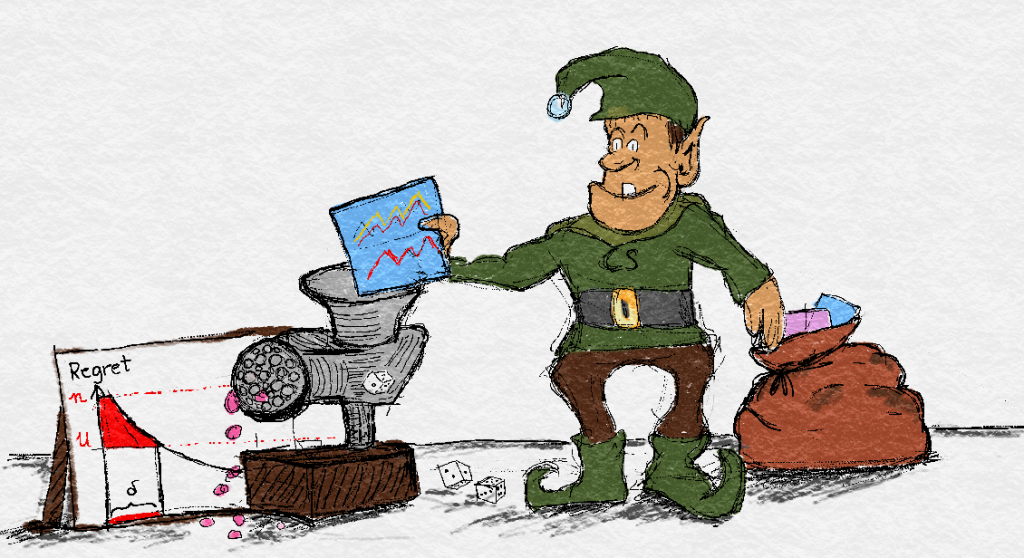
Illustration of the idea of the lower bound proof. An elf randomly chooses a pair of environments from the bag of all possible clipped Gaussian environments and feeds the environment into the policy, which is also randomized. The policy spits out the random regret for both environments. For at least one of the two environments, many of the random regrets will be high with a high chance.
By our earlier remarks, $\hat R_n = \sum_t X_{t1} – \sum_t X_{t,A_t}$ and $\hat R_n’ = \sum_t X_{ti}’ – \sum_t X_{t,A_t}’$. Define $U_t =\one{\eta_t\in [-1/2,1/2-\Delta]}$, $U_t’=\one{\eta_t\in [-1/2,1/2-2\Delta]}$, $A_{tj} = \one{A_t=j}$ and $A_{tj}’ = \one{A_t’=j}$. From \eqref{eq:hplb_rewardgapxt} we see that
\begin{align*}
\hat R_n \ge \Delta\, \sum_t \one{A_t\ne 1} U_t =\Delta\, \sum_t (1-A_{t1}) U_t \ge \Delta\,(U – T_1(n)) \ge \Delta\,(U + T_i(n) – n)\,,
\end{align*}
where we also defined $U = \sum_t U_t$ and used that $T_1(n)+T_i(n)\le n$. Note that $U_t=1$ indicates that $(X_{tj})_j$ are “unclipped”. Similarly, from \eqref{eq:hplb_rewardgapxtp} we see that
\begin{align*}
\hat R_n’ \ge \Delta \, \sum_t \one{A_t’\ne i} U_t’ =\Delta\, \sum_t (1-A_{ti}’) U_t’ \ge \Delta\,( U’ – T_i'(n)) \,,
\end{align*}
where $T_i'(n)=\sum_t A_{ti}’$ and $U’ = \sum_t U_t’$. Based on the lower bounds on $\hat R_n$ and $\hat R_n’$ we thus see that if $T_i(n)\ge n/2$ and $U\ge 3n/4$ then $\hat R_n \ge u\doteq \frac{n\Delta}{4}$ and if $T_i'(n) < n/2$ and $U'\ge 3n/4$ then $\hat R_n' \ge u$ holds, too. Thus, from union bounds,
\begin{align*}
\Probng{ \hat R_n \ge u } &\ge \Prob{ T_i(n)\ge n/2, U\ge 3n/4 } \ge \Prob{ T_i(n)\ge n/2 } - \Prob{U < 3n/4}\,,\\
\Probng{ \hat R_n' \ge u } &\ge \Prob{ T_i'(n) < n/2, U'\ge 3n/4 } \ge \Prob{ T_i'(n) < n/2 } - \Prob{U' < 3n/4}\,.
\end{align*}
Noticing that $U'\le U$ and hence $\Prob{U<3n/4}\le \Prob{U' <3n/4}$, we get
\begin{align*}
\max(\Probng{ \hat R_n \ge u },\Probng{ \hat R_n' \ge u })
& \ge \frac12 \Bigl(\Prob{ T_i(n)\ge n/2 } + \Prob{ T_i'(n) < n/2 }\Bigr) - \Prob{U' < 3n/4}\,.
\end{align*}
The sum $\Prob{ T_i(n)\ge n/2 } + \Prob{ T_i'(n) < n/2 }$ will be lower bounded with the help of the high-probability Pinsker inequality. For an upper bound on $\Prob{U’ < 3n/4}$, we have the following technical lemma:
Lemma (Control of the number of unclipped rounds): Assume that $\Delta\le 1/8$. If $n \ge 32 \log(2/\delta)$ and $\sigma\le 1/10$ then $\Prob{U’<3n/4} \le \delta/2$.
The proof is based on bounding the tail probability of the mean the i.i.d. $(U_t’)_t$ Bernoulli variables using Hoeffding’s inequality and is given later. Intuitively, it is clear that by making $\sigma^2$ small, the number of times $\eta_t$ falls inside $[-1/2,1/4]\subset [-1/2,1/2-2\Delta]$ can be made arbitrary high with arbitrary high probability.
Our goal now is to lower bound $\Prob{ T_i(n)\ge n/2 } + \Prob{ T_i'(n) < n/2 }$ by $3\delta$. As suggested before, we aim to use the high-probability Pinsker inequality. One difficulty that we face is that the events $\{T_i(n)\ge n/2\}$ and $\{T_i'(n) < n/2\}$ may not be complementary as they are defined in terms of a potentially distinct set of random variables. This will be overcome by rewriting the above probabilities using the canonical bandit probability spaces. In fact, we will use the non-extended version of these probability spaces (as defined earlier in the context of stochastic bandits). The reason of this is that after Pinsker, we plan to apply the divergence decomposition identity, which decomposes the divergence between distributions of action-reward sequences.
To properly write things let $Q_j$ denote the distribution of $X_{tj}$ and similarly let $Q_j’$ be the distribution of $X_{tj}’$. These are well defined (why?). Define the stochastic bandits $\beta=(Q_1,\dots,Q_K)$ and $\beta’=(Q’_1,\dots,Q’_K)$. Let $\Omega_n = ([K]\times \R)^n$ and let $\tilde Y_t,\tilde A_t:\Omega_n \to \R$ be the usual coordinate projection functions: $\tilde Y_t(a_1,y_1,\dots,a_n,y_n) = y_t$ and $\tilde A_t(a_1,y_1,\dots,a_n,y_n)=a_t$. Also, let $\tilde T_i(n) = \sum_{t=1}^n \one{\tilde A_t=i}$. Recall that $\PP_{\beta,\pi}$ denotes the probability measure over $\Omega_n$ that arises from the interaction of $\pi$ and $\beta$ (detto for $\PP_{\beta’,\pi}$). Now, since $T_i(n)$ is only a function of $(A_1,X_{1,A_1},\dots,A_n,X_{n,A_n})$ whose probability distribution is exactly $\PP_{\beta,\pi}$, we have
\begin{align*}
\Prob{ T_i(n) \ge n/2 } = \PP_{\beta,\pi}( \tilde T_i(n) \ge n/2 )\,.
\end{align*}
Similarly,
\begin{align*}
\Prob{ T_i'(n) < n/2 } = \PP_{\beta',\pi}( \tilde T_i(n) < n/2 )\,.
\end{align*}
Now, by the high-probability Pinsker inequality and the divergence decomposition lemma,
\begin{align*}
\Prob{ T_i(n) \ge n/2 } + \Prob{ T_i'(n) < n/2 }
& =
\PP_{\beta,\pi}( \tilde T_i(n) \ge n/2 ) + \PP_{\beta',\pi}( \tilde T_i(n) < n/2 ) \\
& \ge
\frac12 \exp\left(- \KL( \PP_{\beta,\pi}, \PP_{\beta',\pi} ) \right) \\
& =
\frac12 \exp\left(- \E_{\beta,\pi}[\tilde T_i(n)] \KL( Q_i, Q_i' ) \right) \\
& \ge
\frac12 \exp\left(- \EE{ T_i(n) } \KL( \mathcal N(\tfrac12,\sigma^2), \mathcal N(\tfrac12 + 2\Delta,\sigma^2) ) \right)\,,
\end{align*}
where in the last equality we used that $Q_j=Q_j'$ unless $j=i$, while in the last step we used $\E_{\beta,\pi}[\tilde T_i(n)] = \EE{ T_i(n) }$ and also that $\KL( Q_i, Q_i' ) \le \KL( \mathcal N(\tfrac12,\sigma^2), \mathcal N(\tfrac12 + 2\Delta,\sigma^2) )$. From where does the last inequality come, one might ask. The answer is the truncation, which always reduces information. More precisely, let $P$ and $Q$ be probability measures on the same probability space $(\Omega, \cF)$. Let $X:\Omega \to \R$ be a random variable and $P_X$ and $Q_X$ be the laws of $X$ with under $P$ and $Q$ respectively. Then $\KL(P_X, Q_X) \leq \KL(P, Q)$.
Now, by the choice of $i$,
\begin{align*}
\EE{ T_i(n) } \KL( \mathcal N(\tfrac12,\sigma^2), \mathcal N(\tfrac12 + 2\Delta,\sigma^2)
\le \frac{n}{K-1} \frac{2\Delta^2}{\sigma^2}\,.
\end{align*}
Plugging this into the previous display we get that if
\begin{align*}
\Delta = \sigma \sqrt{\frac{K-1}{2n} \log\frac{1}{6\delta}}
\end{align*}
then $\Prob{ T_i(n) \ge n/2 } + \Prob{ T_i'(n) < n/2 }\ge 3\delta$ and thus $\max(\Prob{ \hat R_n \ge u },\Prob{ \hat R_n'\ge u} )\ge \delta$. Recalling the definition $u = n\Delta/4$ and choosing $\sigma=1/10$ gives the following result:
Theorem (High probability lower bound for adversarial bandits): Let $K>1$, $n>0$ and $\delta\in (0,1)$ such that
\begin{align*}
n\ge \max\left( 32 \log \frac2{\delta}, (0.8)^2 \frac{K-1}{2} \log \frac{1}{6\delta}\right)
\end{align*}
holds. Then, for any bandit policy $\pi$ there exists a reward sequence $\nu = (x_1,\dots,x_n)\in [0,1]^{nK}$ such that if $\hat R_n$ is the random regret of $\pi$ when interacting with the environment $\nu$ then
\begin{align*}
\Prob{ \hat R_n \ge 0.025\sqrt{\frac{n(K-1)}{2}\log \frac{1}{6\delta}} } \ge \delta\,.
\end{align*}
So what can one take away from this post? The main thing is to recognize that the upper bounds we proved in the previous post cannot be improved very much, at least in this worst case sense. This includes the important difference between the high-probability regret that is achievable when the confidence level $\delta$ is chosen in advance and what is possible if a single strategy must satisfy a high-probability regret guarantee for all confidence levels simultaneously.
Besides this result we also introduced some new techniques that will be revisited in the future, especially the randomization device lemma. The advantage of using clipped and correlated Gaussian rewards is that it ensures the same arm is always optimal, no matter how the noise behaves.
Technicalities
The purpose of this section is to lay to rest the two technical results required in the main body. The first a proof of the lemma which gives us the randomization technique or “device” and afterwards the proof of the proof of the lemma that controls the number of unclipped rounds.
Proof of the randomization device lemma
The argument underlying this goes as follows: If $A=(A_1,\dots,A_n)\in [K]^n$ are the actions of a stochastic policy $\pi=(\pi_1,\dots,\pi_n)$ when interacting with the environment where the rewards $X=(X_1,\dots,X_n)\in \R^{nK}$ are drawn from $Q$ then for $t=1,\dots,n$, $A_t\sim \pi_t(\cdot|A_1,X_{1,A_1},\dots,A_{t-1},X_{t-1,A_{t-1}})$ and thus the distribution $\PP_{Q,\pi}$ of $(X,A)$ satisfies
\begin{align*}
d\PP_{Q,\pi}(x,a)
&= \pi(a|x) d\rho^{\otimes n}(a) dQ(x) \,,
\end{align*}
where $a=(a_1,\dots,a_n)\in [K]^n$, $x\in (x_1,\dots,x_n)\in \R^{nK}$,
\begin{align*}
\pi(a|x)\doteq
\pi_1(a_1) \pi_2(a_2|a_1,x_{1,a_1}) \cdots \pi_n(a_n|a_1,x_{1,a_1}, \dots,a_{n-1},x_{n-1,a_{n-1}})
\end{align*}
and $\rho^{\otimes n}$ is the $n$-fold product $\rho$ with itself, where $\rho$ is the counting measure $\rho$ on $[K]$. Letting $\delta_x$ be the Dirac (probability) measure on $\R^{nK}$ concentrated at $x$ (i.e., $\delta_x(U) = \one{x\in U}$), we have that $\PP_{Q,\pi}$ can be disintegrated into $Q$ and $\{\PP_{\delta_x,\pi}\}_x$. In particular, a direct calculation verifies that
\begin{align}
d\PP_{Q,\pi}(x,a) = \int_{y\in \R^{nK}} dQ(y) \, d\PP_{\delta_y,\pi}(x,a) \,.
\label{eq:disintegration}
\end{align}
Let $(X_t,A_t)$ be the reward and action of round $t$ in the extended canonical bandit probability space and $\hat R_n$ the random regret defined in terms of these random variables. For any Borel $U\subset \R$,
\begin{align*}
\PP_{Q,\pi}( \hat R_n \in U )
&= \int \one{\hat R_n(x,a)\in U} d\PP_{Q,\pi}(x,a) \\
&= \int_{\R^{nK}} dQ(y) \left( \int_{\R^{nK}\times [K]^n} \one{\hat R_n(x,a)\in U} d\PP_{\delta_y,\pi}(x,a) \right)\\
&= \int_{\R^{nK}} dQ(y) \PP_{\delta_y,\pi}( \hat R_n\in U )\,,
\end{align*}
where the the second equality uses \eqref{eq:disintegration} and Fubini. From the above equality it is obvious that it is not possible that $\PP_{Q,\pi}( \hat R_n \in U )\ge \delta$ while for all $y\in \mathrm{support}(Q)$, $\PP_{\delta_y,\pi}( \hat R_n\in U )<\delta$, thus finishing the proof.
QED
Proof of lemma controlling number of clipped rounds: First note that $U’\le U$ and thus $\Prob{U < 3n/4}\le \Prob{U '< 3n/4}$ hence it suffices to control the latter.
Since $\Delta\le 1/8$ and $\eta_t$ is a Gaussian with zero mean and variance $\sigma^2$, and in particular $\eta_t$ is $\sigma^2$-subgaussian, we have
\begin{align*}
1 - p = \Prob{U_t' = 0}
& \leq \Prob{ |\eta_t| > 1/2-2\Delta }
\leq 2 \exp\left(-\frac{\left(1/2 – 2\Delta\right)^2}{2\sigma^2}\right)\\
& \leq 2 \exp\left(-\frac{1}{2 (4)^2 \sigma^2}\right)
\le \frac{1}{8}\,,
\end{align*}
where the last inequality follows whenever $\sigma^2 \le \frac{1}{32 \log 16}$ which is larger than $0.01$. Therefore $p \ge 7/8$ and
\begin{align*}
\Prob{\sum_{t=1}^n U_t’ < \frac{3n}{4}}
&= \Prob{\frac{1}{n} \sum_{t=1}^n ( U_t' - p) < -(p-\frac{3}{4}) } \\
&\le \Prob{\frac{1}{n} \sum_{t=1}^n ( U_t' - p) \le - \frac{1}{8}} \\
&\leq \exp\left(-\frac{n}{32}\right) \leq \frac{\delta}{2}\,,
\end{align*}
where the second last inequality uses Hoeffding’s bound together with that $U_t’-p$ is $1/4$-subgaussian, and the last holds by our assumption on $n$.
QED
Notes
Note 1: It so happens that the counter-example construction we used means that the same arm has the best reward in every round (not just the best mean). It is perhaps a little surprising that algorithms cannot exploit this fact, in contrast the experts setting where this knowledge enormously improves the achievable regret.
Note 2: Adaptivity is all the rage right now. Can you design an adversarial bandit algorithm that exploits “easy data” when available? For example, if the rewards don’t change much over time, or lie in a small range. There are still a lot of open questions in this area. The paper referenced below gives lower bounds for some of these situations.
References
Sebastien Gerchinovitz and Tor Lattimore. Refined lower bounds for adversarial bandits. 2016

Please, Could you explain why the (2) has upper bound like nδ+O(√Knlog(Kδ))?