
Continuing the previous post, we prove the claimed minimax lower bound.
We start with a useful result that quantifies the difficulty of identifying whether or not an observation is drawn from similar distributions $P$ and $Q$ defined over the same measurable space $(\Omega,\cF)$. In particular, the difficulty will be shown to increase as a function of the relative entropy of $P$ with respect to $Q$. In the result below, as usual in probability theory, for $A\subset \Omega$, $A^c$ denotes the complement of $A$ with respect to $\Omega$: $A^c = \Omega \setminus A$.
Theorem (High-probability Pinsker): Let $P$ and $Q$ be probability measures on the same measurable space $(\Omega, \cF)$ and let $A \in \cF$ be an arbitrary event. Then,
\begin{align}\label{eq:pinskerhp}
P(A) + Q(A^c) \geq \frac{1}{2}\, \exp\left(-\KL(P, Q)\right)\,.
\end{align}
The logic of the result is as follows: If $P$ and $Q$ are similar to each other (e.g., in the sense that $\KL(P,Q)$ is small) then for any event $A\in \cF$, $P(A)\approx Q(A)$ and $P(A^c) \approx Q(A^c)$. Since $P(A)+P(A^c)=1$, we thus also expect $P(A)+Q(A^c)$ to be “large”. How large is “large” is the contents of the result. In particular, using $2 \max(a,b)\ge a+b$, it follows that for any $0<\delta\le 1$, to guarantee $\max(P(A),Q(A^c))\le \delta$, it is necessary that $\KL(P,Q)\ge \log(\frac{1}{4\delta})$, that is relative entropy of $P$ with respect to $Q$ must be larger than the right-hand side. Connecting the dots, this means that the information coming from an observation drawn from $P$ relative to expecting an observation from $Q$ must be just large enough.
Note that if $P$ is not absolutely continuous with respect to $Q$ then $\KL(P,Q)=\infty$ and the result is vacuous. Also note that the result is symmetric. We could replace $\KL(P, Q)$ with $\KL(Q, P)$, which sometimes leads to a stronger result because the relative entropy is not symmetric.
This theorem is useful for proving lower bounds because it implies that at least one of $P(A)$ and $Q(A^c)$ is large. Then, in an application where after some observations a decision needs to be made, $P$ and $Q$ are selected such that the a correct decision under $P$ is incorrect under $Q$ and vice versa. Then one lets $A$ be the event when the decision is incorrect under $P$ and $A^c$ is the event that the decision is incorrect under $Q$. The result then tells us that it is impossible to design a decision rule such that the probability of an incorrect decision is small under both $P$ and $Q$.
To illustrate this, consider the normal means problem when $X\sim N(\mu,1)$ is observed with $\mu \in \{0,\Delta\}$. In this case, we let $P$ the distribution of $X$ under $\mu=0$, $Q$ the distribution of $X$ under $\mu=\Delta$ and if $f: \R \to \{0,\Delta\}$ is the measurable function that is proposed as the decision rule, $A = \{\, x\in \R \,: f(x) \ne 0 \}$. Then, using e.g. $\Delta=1$, the theorem tells us that
\begin{align*}
P(A) + Q(A^c) \geq \frac{1}{2}\, \exp\left(-\KL(P, Q)\right)
= \frac{1}{2}\, \exp\left(-\frac{\Delta^2}{2\sigma^2}\right)
= \frac{1}{2}\, \exp\left(-1/2\right) \geq 3/10\,.
\end{align*}
This means that no matter how we chose our decision rule $f$, we simply do not have enough data to make a decision for which the probability of error on either $P$ or $Q$ is smaller than $3/20$. All that remains is to apply this idea to bandits and we will have our lower bound. The proof of the above result is postponed to the end of the post.
After this short excursion into information theory, let us return to the world of $K$-action stochastic bandits. In what follows we fix $n>0$, the number of rounds and $K>0$, the number of actions. Recall that given a $K$-action bandit environment $\nu = (P_1,\dots,P_K)$ ($P_i$ is the distribution of rewards for action $i$) and a policy $\pi$, the outcome of connecting $\pi$ and $\nu$ was defined as the random variables $(A_1,X_1,\dots,A_n,X_n)$ such that for $t=1,2,\dots,n$, the distribution of $A_t$ given the history $A_1,X_1,\dots,A_{t-1},X_{t-1}$ is uniquely determined by the policy $\pi$, while the distribution of $X_t$ given the history $A_1,X_1,\dots,A_{t-1},X_{t-1},A_t$ was required to be $P_{A_t}$. While the probability space $(\Omega,\cF,\PP)$ that carries these random variables can be chosen in many different ways, you should convince yourself that the constraints mentioned uniquely determine the distribution of the random element $H_n = (A_1,X_1,\dots,A_n,X_n)$ (or wait two paragraphs). As such, despite that $(\Omega,\cF,\PP)$ is non-unique, we can legitimately define $\PP_{\nu,\pi}$ to be the distribution of $H_n$ (suppressing dependence on $n$).
In fact, we will find it useful to write this distribution with a density. To do this, recall from the Radon-Nykodim theorem that if $P,Q$ are measures over a common measurable space $(\Omega,\cF)$ such that $Q$ is $\sigma$-finite and $P\ll Q$ (i.e., $P$ is absolutely continuous w.r.t. $Q$, which is sometimes written as $Q$ dominates $P$) then there exists a random variable $f:\Omega \to \R$ such that
\begin{align}\label{eq:rnagain}
\int_A f dQ = \int_A dP, \qquad \forall A\in \cF\,.
\end{align}
The function $f$ is said to be the density of $P$ with respect to $Q$, also denoted by $\frac{dP}{dQ}$. Since writing $\forall A\in \cF$, $\int_A \dots = \int_A \dots $ is a bit redundant, to save typing, following standard practice, in the future we will write $f dQ = dP$ (or $f(\omega) dQ(\omega) = dP(\omega)$ to detail the dependence on $\omega\in \Omega$) as a shorthand for $\eqref{eq:rnagain}$. This also explains why we write $f = \frac{dP}{dQ}$.
With this, it is not hard to verify that for any $(a_1,x_1,\dots,a_n,x_n)\in \cH_n \doteq ([K]\times \R)^n$ we have
\begin{align}
\begin{split}
d\PP_\nu(a_1,x_1,\dots,a_n,x_n)
& = \pi_1(a_1) p_{a_1}(x_1) \, \pi_2(a_2|a_1,x_1) p_{a_2}(x_2)\cdot \\
& \quad \cdots \pi_n(a_n|a_1,x_1,\dots,a_{n-1},x_{n-1} )\,p_{a_n}(x_n) \\
& \qquad \times d\lambda(x_1) \dots d\lambda(x_n) d\rho(a_1) \dots d\rho(a_n)\, ,
\end{split}
\label{eq:jointdensity}
\end{align}
where
- $\pi = (\pi_t)_{1\le t \le n}$ with $\pi_t(a_t|a_1,x_1,\dots,a_{t-1},x_{t-1})$ being the probability that policy $\pi$ in round $t$ chooses action $a_t\in [K]$ when the sequence of actions and rewards in the previous rounds are $(a_1,x_1,\dots,a_{t-1},x_{t-1})\in \cH_{t-1}$;
- $p_i$ is defined by $p_i d\lambda = d P_i$, where $\lambda$ is a common dominating measure for $P_1,\dots,P_K$, and
- $\rho$ is the counting measure on $[K]$: For $A\subset [K]$, $\rho(A) = |A \cap [K]|$.
There is no loss of generality in assuming that $\lambda$ exist: For example, we can always use $\lambda = P_1+\dots+P_K$. In a note at the end of the post, for full mathematical rigor, we add another condition to the definition of $\pi$. (Can you guess what this condition should be?)
Note that $\PP_{\nu,\pi}$, as given by the right-hand side of the above displayed equation, is a distribution over $(\cH_n,\cF_n)$ where $\cF_n=\mathcal L(\R^{2n})|_{\cH_n}$. Here, $\mathcal L(\R^{2n})$ is the Lebesgue $\sigma$-algebra over $\R^{2n}$ and $\mathcal L(\R^{2n})|_{\cH_n}$ is its restriction to $\cH_n$.
As mentioned in the previous post, given any two bandit environments, $\nu=(P_1,\dots,P_K)$ and $\nu’=(P’_1,\dots,P’_K)$, we expect $\PP_{\nu,\pi}$ and $\PP_{\nu’,\pi}$ to be close to each other if all of $P_i$ and $P_i’$ are close to each other, regardless of the policy $\pi$ (a sort of continuity result). Our next result will make this precise; in fact we will show an identity that expresses $\KL( \PP_{\nu,\pi}, \PP_{\nu’,\pi})$ as a function $\KL(P_i,P’_i)$, $i=1,\dots,K$.
Before stating the result, we need to introduce the concept of ($n$-round $K$-action) canonical bandit models. The idea is to fix the measurable space $(\Omega,\cF)$ (that holds the variables $(X_t,A_t)_t$) in a special way. In particular, we set $\Omega=\cH_n$ and $\cF=\cF_n$. Then, we define $A_t,X_t$, $t=1,\dots,n$ to be the coordinate projections:
\begin{align}
\begin{split}
A_t( a_1,x_1,\dots,a_n,x_n ) &= a_t\,, \text{ and }\\
X_t( a_1,x_1,\dots,a_n,x_n) &= x_t,\, \quad \forall t\in [n]\,\text{ and } \forall (a_1,x_1,\dots,a_n,x_n)\in \cH_n\,.
\end{split}
\label{eq:coordproj}
\end{align}
Now, given some policy $\pi$ and bandit environment $\nu$, if we set $\PP=\PP_{\nu,\pi}$ then, trivially, the distribution of $H_n=(A_1,X_1,\dots,A_n,X_n)$ is indeed $\PP_{\nu,\pi}$ as expected. Thus, $A_t,X_t$ as defined by $\eqref{eq:coordproj}$, satisfies the requirements we posed against the random variables that describe the outcome of the interaction of a policy and an environment. However, $A_t,X_t$ are fixed, no matter the choice of $\nu,\pi$. This is in fact the reason why it is convenient to use the canonical bandit model! Furthermore, since all our past and future statements concern only the properties of $\PP_{\nu,\pi}$ (and not the minute details of the definition of the random variables $(A_1,X_1,\dots,A_n,X_n)$), there is no loss of generality in assuming that in all our expressions $(A_1,X_1,\dots,A_n,X_n)$ is in fact defined over the canonical bandit model using $\eqref{eq:coordproj}$. (We avoided initially the canonical model because up to now there was no advantage to introducing and using it.)
Before we state our promised result, we introduce one last notation that we need: Since we use the same measurable space $(\cH_n,\cF_n)$ with multiple environments $\nu$ and policies $\pi$, which give rise to various probability measures $\PP = \PP_{\nu,\pi}$, when writing expectations we will index $\E$ the same way as $\PP$ is indexed. Thus, $\E_{\nu,\pi}$ denotes expectation underlying $\PP_{\nu,\pi}$ (i.e., $\E_{\nu,\pi}[X] = \int X d\PP_{\nu,\pi}$. When $\pi$ is fixed, we will also drop $\pi$ from the indices and just write $\PP_{\nu}$ (and $\E_{\nu}$) for $\PP_{\nu,\pi}$ (respectively, $\E_{\nu,\pi}$).
With this, we are ready to state the promised result:
Lemma (Divergence decomposition): Let $\nu=(P_1,\ldots,P_K)$ be the reward distributions associated with one $K$-armed bandit, and let $\nu’=(P’_1,\ldots,P’_K)$ be the reward distributions associated with the another $K$-armed bandit. Fix some policy $\pi$ and let $\PP_\nu = \PP_{\nu,\pi}$ and $\PP_{\nu’} = \PP_{\nu’,\pi}$ be the distributions induced by the interconnection of $\pi$ and $\nu$ (respectively, $\pi$ and $\nu’$). Then
\begin{align}
\KL(\PP_{\nu}, \PP_{\nu’}) = \sum_{i=1}^K \E_{\nu}[T_i(n)] \, \KL(P_i, P’_i)\,.
\label{eq:infoproc}
\end{align}
In particular the lemma implies that $\PP_{\nu}$ and $\PP_{\nu’}$ will be close if for all $i$, $P_i$ and $P’_i$ were close. A nice feature of the lemma is that it provides not only a bound on the divergence of $\PP_{\nu}$ from $\PP_{\nu’}$, but it actually expresses this with an identity.
Proof
First, assume that $\KL(P_i,P’_i)<\infty$ for all $i\in [K]$. From this, it follows that $P_i\ll P’_i$. Define $\lambda = \sum_i P_i + P’_i$ and let $p_i = \frac{dP_i}{d\lambda}$ and let $p’_i = \frac{dP’_i}{d\lambda}$. By the chain rule of Radon-Nikodym derivatives, $\KL(P_i,P’_i) = \int p_i \log( \frac{p_i}{p’_i} ) d\lambda$.
Let us now evaluate $\KL( \PP_{\nu}, \PP_{\nu’} )$. By the fundamental identity for the relative entropy, this is equal to $\E_\nu[ \log \frac{d\PP_\nu}{d\PP_{\nu’}} ]$, where $\frac{d\PP_\nu}{d\PP_{\nu’}}$ is the Radon-Nikodym derivative of $\PP_\nu$ with respect to $\PP_{\nu’}$. It is easy to see that both $\PP_\nu$ and $\PP_{\nu’}$ can be written in the form given by $\eqref{eq:jointdensity}$ (this is where we use that $\lambda$ dominates all of $P_i$ and $P_i’$). Then, using the chain rule we get
\begin{align*}%\label{eq:logrn}
\log \frac{d\PP_\nu}{d\PP_{\nu’}} = \sum_{t=1}^n \log \frac{p_{A_t}(X_t)}{p’_{A_t}(X_t)}\,
\end{align*}
(the terms involving the policy cancel!). Now, taking expectations of both sides, we get
\begin{align*}
\E_{\nu}\left[ \log \frac{d\PP_\nu}{d\PP_{\nu’}} \right]
= \sum_{t=1}^n \E_{\nu}\left[ \log \frac{p_{A_t}(X_t)}{p’_{A_t}(X_t)} \right]\,,
\end{align*}
and
\begin{align*}
\E_{\nu}\left[ \log \frac{p_{A_t}(X_t)}{p’_{A_t}(X_t)} \right]
& = \E_{\nu}\left[ \E_{\nu}\left[\log \frac{p_{A_t}(X_t)}{p’_{A_t}(X_t)} \, \big|\, A_t \right] \, \right]
= \E_{\nu}\left[ \KL(P_{A_t},P’_{A_t}) \right]\,,
\end{align*}
where in the second equality we used that under $\PP_{\nu}$, conditionally on $A_t$, the distribution of $X_t$ is $dP_{A_t} = p_{A_t} d\lambda$. Plugging back into the previous display,
\begin{align*}
\E_{\nu}\left[ \log \frac{d\PP_\nu}{d\PP_{\nu’}} \right]
&= \sum_{t=1}^n \E_{\nu}\left[ \log \frac{p_{A_t}(X_t)}{p’_{A_t}(X_t)} \right] \\
&= \sum_{t=1}^n \E_{\nu}\left[ \KL(P_{A_t},P’_{A_t}) \right] \\
&= \sum_{i=1}^K \E_{\nu}\left[ \sum_{t=1}^n \one{A_t=i} \KL(P_{A_t},P’_{A_t}) \right] \\
&= \sum_{i=1}^K \E_{\nu}\left[ T_i(n)\right]\KL(P_{i},P’_{i})\,.
\end{align*}
When the right-hand side of $\eqref{eq:infoproc}$ is infinite, by our previous calculation, it is not hard to see that the left-hand side will also be infinite.
QED
Using the previous theorem and lemma we are now in a position to present and prove the main result of the post, a worst-case lower bound on the regret of any algorithm for finite-armed stochastic bandits with Gaussian noise. Recall that previously we used $\cE_K$ to denote the class of $K$ action bandit environments where the reward distributions have means in $[0,1]^K$ and the noise in the rewards have 1-subgaussian tails. Denote by $G_\mu\in \cE_K$ the bandit environment where all distributions are Gaussian with unit variance and the vector of means is $\mu\in [0,1]^K$. To make the dependence of the regret on the policy and the environment explicit, in accordance with the notation of the previous post, we will use $R_n(\pi,E)$ to denote the regret of policy $\pi$ on a bandit instance $E$.
Theorem (Worst-case lower bound): Fix $K>1$ and $n\ge K-1$. Then, for any policy $\pi$ there exists a mean vector $\mu \in [0,1]^K$ such that
\begin{align*}
R_n(\pi,G_\mu) \geq \frac{1}{27}\sqrt{(K-1) n}\,.
\end{align*}
Since $G_\mu \in \cE_K$, it follows that the minimax regret for $\cE_K$ is lower bounded by the right-hand side of the above display as soon as $n\ge K-1$:
\begin{align*}
R_n^*(\cE_K) \geq \frac{1}{27}\sqrt{(K-1) n}\,.
\end{align*}
The idea of the proof is illustrated on the following figure:
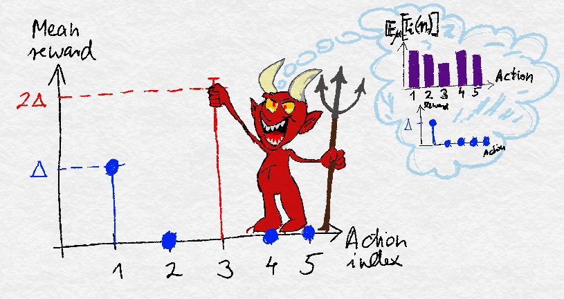
The idea of the minimax lower bound. Given the policy and one environment, the evil antagonist picks another environment so that the policy will suffer a large regret in at least one of the environments.
Proof
Fix a policy $\pi$. Let $\Delta\in [0,1/2]$ be some constant to be chosen later. As described in the previous post, we choose two Gaussian environments with unit variance. In the first environment, the vector of means of the rewards per arm is
\begin{align*}
\mu = (\Delta, 0, 0, \dots,0)\,.
\end{align*}
This environment and $\pi$ gives rise to the distribution $\PP_{G_\mu,\pi}$ on the canonical bandit model $(\cH_n,\cF_n)$. For brevity, we will use $\PP_{\mu}$ in place of $\PP_{G_\mu,\pi}$. The expectation under $\PP_{\mu}$ will be denoted by $\E_{\mu}$. Recall that on measurable space $(\cH_n,\cF_n)$, $A_t,X_t$ are just the coordinate projections defined using $\eqref{eq:coordproj}$.
To choose the second environment, pick
\begin{align*}
i = \argmin_{j\ne 1} \E_{\mu}[ T_j(n) ]\,.
\end{align*}
Note that $\E_{\mu}[ T_i(n) ] \le n/(K-1)$ because otherwise we would have $\sum_{j\ne 1} \E_{\mu}[T_j(n)]>n$, which is impossible. Note also that $i$ depends on $\pi$. The second environment has means
\begin{align*}
\mu’ = (\Delta,0,0, \dots, 0, 2\Delta, 0, \dots, 0 )\,,
\end{align*}
where specifically $\mu’_i = 2\Delta$. In particular, $\mu_j = \mu’_j$ except at index $i$. Note that the optimal action in $G_{\mu}$ is action one, while the optimal action in $G_{\mu’}$ is action $i\ne 1$. We again use the shorthand $\PP_{\mu’} = \PP_{G_{\mu’},\pi}$.
Intuitively, if $\pi$ chooses action one infrequently while interacting with $\mu$ (i.e., if $T_1(n)$ is small with high probability), then $\pi$ should do poorly in $G_{\mu}$, while if it chooses action one frequently while interacting with $G_{\mu’}$, then it will do poorly in $G_{\mu’}$. In particular, by the basic regret decomposition identity and a simple calculation,
\begin{align*}
R_n(\pi,G_\mu) %= \E_\mu[ (n-T_1(n)) \Delta ] \ge \E_\mu[ \one{T_1(n)\le n/2} ]\, \left(n-\frac{n}{2}\right)\, \Delta =
\ge \PP_{\mu}(T_1(n)\le n/2) \frac{n\Delta}{2}\, \quad \text{and} \quad
R_n(\pi,G_{\mu’}) > \PP_{\mu’}(T_1(n)> n/2)\, \frac{n\Delta}{2}\,.
%R_n(\pi,G_{\mu’}) %\ge \E_{\mu’}[ T_1(n) \Delta ] > \E_{\mu’}[ \one{T_1(n)> n/2} ]\, \frac{n\Delta}{2} =
%\ge \PP_{\mu’}(T_1(n)> n/2)\, \frac{n\Delta}{2}\,.
\end{align*}
Chaining this with the high-probability Pinsker inequality,
\begin{align*}
R_n(\pi,G_\mu) + R_n(\pi,G_{\mu’})
& > \frac{n\Delta}{2}\,\left( \PP_{\mu}(T_1(n)\le n/2) + \PP_{\mu’}(T_1(n)> n/2) \right) \\
& \ge \frac{n\Delta}{4}\, \exp( – \KL(\PP_{\mu},\PP_{\mu’}) )\,.
\end{align*}
It remains to upper bound $\KL(\PP_{\mu},\PP_{\mu’})$, i.e., to show that $\PP_\mu$ and $\PP_{\mu’}$ are indeed not far. For this, we use the divergence decomposition lemma, the definitions of $\mu$ and $\mu’$ and then exploit the choice of $i$ to get
\begin{align*}
\KL(\PP_\mu, \PP_{\mu’}) = \E_{\mu}[T_i(n)] \KL( \mathcal N(0,1), \mathcal N(2\Delta,1) ) =
\E_{\mu}[T_i(n)]\, \frac{(2\Delta)^2}{2} \leq \frac{2n\Delta^2}{K-1} \,.
\end{align*}
Plugging this into the previous display, we find that
\begin{align*}
R_n(\pi,G_\mu) + R_n(\pi,G_{\mu’}) \ge \frac{n\Delta}{4}\, \exp\left( – \frac{2n\Delta^2}{K-1} \right)\,.
\end{align*}
The result is completed by tuning $\Delta$. In particular, the optimal choice for $\Delta$ happens to be $\Delta = \sqrt{(K-1)/4n}$, which is below $1/2$ when $n$ is large compared to $K$, as postulated in the conditions of the theorem. The final steps are lower bounding $\exp(-1/2)$ and using $2\max(a,b) \ge a+b$.
QED
This concludes the proof of the worst-case lower bound, showing that no algorithm can do better than $O(\sqrt{nK})$ over all problems simultaneously. Coming in the next post we will show that the asymptotic logarithmic regret of UCB is essentially not improvable when the noise is Gaussian.
In the remainder of the post, we give the proof of the “high probability” Pinsker inequality, followed by miscellaneous thoughts.
Proof of the Pinsker-type inequality
It remains to show the proof of the Pinsker-type inequality stated above. In the proof, to save space, we use the convention of denoting the minimum of $a$ and $b$ by $a\wedge b$, while we denote their maximum by $a \vee b$.
If $\KL(P,Q)=\infty$, there is nothing to be proven. On the other hand, by our previous theorem on relative entropy, $\KL(P,Q)<\infty$ implies that $P \ll Q$. Take $\nu = P+Q$. Note that $P,Q\ll \nu$. Hence, we can define $p = \frac{dP}{d\nu}$ and $q = \frac{dQ}{d\nu}$ and use the chain rule for Radon-Nikodym derivatives to derive that $\frac{dP}{dQ} \frac{dQ}{d\nu} = \frac{dP}{d\nu}$, or $\frac{dP}{dQ} = \frac{\frac{dP}{d\nu}}{\frac{dQ}{d\nu}}$. Thus,
\begin{align*}
\KL(P,Q) = \int p \log(\frac{p}{q}) d\nu\,.
\end{align*}
For brevity, when writing integrals with respect to $\nu$, in this proof, we will drop $d\nu$. Thus, we will write, for example $\int p \log(p/q)$ for the above integral.
Instead of $\eqref{eq:pinskerhp}$, we prove the stronger result that
\begin{align}\label{eq:pinskerhp2}
\int p \wedge q \ge \frac12 \, \exp( – \KL(P,Q) )\,.
\end{align}
This indeed is sufficient since $\int p \wedge q = \int_A p \wedge q + \int_{A^c} p \wedge q \le \int_A p + \int_{A^c} q = P(A) + Q(A^c)$.
We start with an inequality attributed to Lucien Le Cam, which lower bounds the left-hand side of $\eqref{eq:pinskerhp2}$. The inequality states that
\begin{align}\label{eq:lecam}
\int p \wedge q \ge \frac12 \left( \int \sqrt{pq} \right)^2\,.
\end{align}
Starting from the right-hand side above, using $pq = (p\wedge q) (p \vee q)$ and then Cauchy-Schwartz, we get
\begin{align*}
\left( \int \sqrt{pq} \right)^2
= \left(\int \sqrt{(p\wedge q)(p\vee q)} \right)^2
\le \left(\int p \wedge q \right)\, \left(\int p \vee q\right)\,.
\end{align*}
Now, using $p\wedge q + p \vee q = p+q$, the proof is finished by substituting $\int p \vee q = 2-\int p \wedge q \le 2$ and dividing both sides by two.
Thus, it remains to lower bound the right-hand side of $\eqref{eq:lecam}$. For this, we use Jensen’s inequality. First, we write $(\cdot)^2$ as $\exp (2 \log (\cdot))$ and then move the $\log$ inside the integral:
\begin{align*}
\left(\int \sqrt{pq} \right)^2 &= \exp\left( 2 \log \int \sqrt{pq} \right)
= \exp\left( 2 \log \int p \sqrt{\frac{q}{p}} \right) \\
&\ge \exp\left( 2 \int p \,\frac12\,\log \left(\frac{q}{p}\right)\, \right) \\
&= \exp\left( 2 \int_{pq>0} p \,\frac12\,\log \left(\frac{q}{p}\right)\, \right) \\
&= \exp\left( – \int_{pq>0} p \log \left(\frac{p}{q}\right)\, \right) \\
&= \exp\left( – \int p \log \left(\frac{p}{q}\right)\, \right)\,.
\end{align*}
Here, in the fourth and the last step we used that since $P\ll Q$, $q=0$ implies $p=0$, hence $p>0$ implies $q>0$, and eventually $pq>0$. Putting together the inequalities finishes the proof.
QED
Notes
Note 1: We used the Gaussian noise model because the KL divergences are so easily calculated in this case, but all that we actually used was that $\KL(P_i, P_i’) = O((\mu_i – \mu_i’)^2)$ when the gap between the means $\Delta = \mu_i – \mu_i’$ is small. While this is certainly not true for all distributions, it very often is. Why is that? Let $\{P_\mu : \mu \in \R\}$ be some parametric family of distributions on $\Omega$ and assume that distribution $P_\mu$ has mean $\mu$. Then assuming the densities are twice differentiable and that everything is sufficiently “nice” that integrals and derivatives can be exchanged (as is almost always the case), we can use a Taylor expansion about $\mu$ to show that
\begin{align*}
\KL(P_\mu, P_{\mu+\Delta})
&\approx \KL(P_\mu, P_\mu) + \left.\frac{\partial}{\partial \Delta} \KL(P_\mu, P_{\mu+\Delta})\right|_{\Delta = 0} \Delta + \frac{1}{2}\left.\frac{\partial^2}{\partial\Delta^2} \KL(P_\mu, P_{\mu+\Delta})\right|_{\Delta = 0} \Delta^2 \\
&= \left.\frac{\partial}{\partial \Delta} \int_{\Omega} \log\left(\frac{dP_\mu}{dP_{\mu+\Delta}}\right) dP_\mu \right|_{\Delta = 0}\Delta
+ \frac12 I(\mu) \Delta^2 \\
&= -\left.\int_{\Omega} \frac{\partial}{\partial \Delta} \log\left(\frac{dP_{\mu+\Delta}}{dP_{\mu}}\right) \right|_{\Delta=0} dP_\mu \Delta
+ \frac12 I(\mu) \Delta^2 \\
&= -\left.\int_{\Omega} \frac{\partial}{\partial \Delta} \frac{dP_{\mu+\Delta}}{dP_{\mu}} \right|_{\Delta=0} dP_\mu \Delta
+ \frac12 I(\mu) \Delta^2 \\
&= – \frac{\partial}{\partial \Delta} \left.\int_{\Omega} \frac{dP_{\mu+\Delta}}{dP_{\mu}} dP_\mu \right|_{\Delta=0} \Delta
+ \frac12 I(\mu) \Delta^2 \\
&= -\left.\frac{\partial}{\partial \Delta} \int_{\Omega} dP_{\mu+\Delta} \right|_{\Delta=0}\Delta
+ \frac12 I(\mu) \Delta^2 \\
&= \frac12 I(\mu)\Delta^2\,,
\end{align*}
where $I(\mu)$, introduced in the second line, is called the Fisher information of the family $(P_\mu)_{\mu}$ at $\mu$. Note that if $\lambda$ is a common dominating measure for $(P_{\mu+\Delta})$ for $\Delta$ small, $dP_{\mu+\Delta} = p_{\mu+\Delta} d\lambda$ and we can write
\begin{align*}
I(\mu) = -\int \left.\frac{\partial^2}{\partial \Delta^2} \log\, p_{\mu+\Delta}\right|_{\Delta=0}\,p_\mu d\lambda\,,
\end{align*}
which is the form that is usually given in elementary texts. The upshot of all this is that $\KL(P_\mu, P_{\mu+\Delta})$ for $\Delta$ small is indeed quadratic in $\Delta$, with the scaling provided by $I(\mu)$, and as a result the worst-case regret is always $O(\sqrt{nK})$, provided the class of distributions considered is sufficiently rich and not too bizarre.
Note 2: In the previous post we showed that the regret of UCB is at most $O(\sqrt{nK \log(n)})$, which does not match the lower bound that we just proved. It is possible to show two things. First, that UCB does not achieve $O(\sqrt{nK})$ regret. The logarithm is real, and not merely a consequence of lazy analysis. Second, there is a modification of UCB (called MOSS) that matches the lower bound up to constant factors. We hope to cover this algorithm in future posts, but the general approach is to use a less conservative confidence level.
Note 3: We have now shown a lower bound that is $\Omega(\sqrt{nK})$, while in the previous post we showed an upper bound for UCB that was $O(\log(n))$. What is going on? Do we have a contradiction? Of course, the answer is no and the reason is that the logarithmic regret guarantees depended on the inverse gaps between the arms, which may be very large.
Note 4: Our lower bounding theorem was only proved when $n$ is at least linear in $K$. What happens when $n$ is small compared to $K$ (in particular, $n\le (K-1)$) above? A careful investigation of the proof of the theorem shows that in this case a linear lower bound of size $n/8\exp(-1/2)$ also holds for the regret (choose $\Delta=1/2$). Note that for small values of $n$ compared to $K$, the square-root lower bound gives larger than linear regret owning to that for $0\le x\le 1$, $\sqrt{x}\ge x$ and if the mean rewards are restricted the $[0,1]$ interval than the regret can not be larger than $n$, i.e., for $n$ small, the lower bound is vacuous (in particular, this happens when $n\le (K-1)/27$). Hence, the square-root form is simply too strong to hold for small values of $n$. A lower bound, which joins the two cases and thus holds for any value of $n$ regardless of $K$ is $\frac{\exp(-1/2)}{16}\, \min( n, \sqrt{(K-1)n} )$.
Note 5: To guarantee that the right-hand side of $\eqref{eq:jointdensity}$ defines a measure, we also must have that for any $t\ge 1$, $\pi_t(i|\cdot): \cH_{t-1} \to [0,1]$ is a measurable map. In fact, $\pi_t$ is a simple version of a so-called probability kernel. For the interested reader, we add the general definition for a probability kernel $K$: Let $(\cX,\cF)$, $(\cY,\cG)$ be a measurable spaces. $K:\cX \times \cG \to [0,1]$ is a probability kernel if it satisfies the following two properties: (i) For any $x\in \cX$, $K(x,\cdot)$ as the $U \mapsto K(x,U)$ ($U\in \cG$) map is a probability measure; (ii) For any $U\in \cG$, $K(\cdot,U)$ as the $x\mapsto K(x,U)$ ($x\in \cX$) map is measurable. When $\cY$ is finite and $\cG= 2^{\cY}$, instead of $K(x,U)$ for $U\subset \cY$, it is common that we specify the values of $K(x,\{y\})$ for $x\in \cX$ and $y\in \cY$ and in these cases we also often write $K(x,y)$. It is also common to write $K(U|x)$ (or in the discrete case $K(y|x)$).
Note 6: There is another subtlety in connection to the definition of $\PP_{\nu,\pi}$ is that we emphasized that $\lambda$ should be a measure over the Lebesgue $\sigma$-algebra $\mathcal L(\R)$. This will be typically easy to satisfy and holds for example when $P_1,\dots,P_K$ are defined over $\mathcal L(\R)$. This requirement would not be needed though if we did not insist on using the canonical bandit model. In particular, by their original definition, $X_1,\dots,X_n$ (as maps from $\Omega$ to $\R$) need only be $\cF/\mathcal B(\R)$ measurable (where $\mathcal B(\R)$ is the Borel $\sigma$-algebra over $\R$) and thus at a first sight it may seem strange to require that $P_1,\dots,P_K$ are defined over $\mathcal L(\R)$. The reason we require this is because in the canonical model we wish to use the Lebesgue $\sigma$-algebra of $\R^{2n}$ (in particular its restriction to $\cH_n$), which is in fact demanded by our wish to work with complete measure-spaces. This latter, as explained at the link, is useful because it essentially allows us not to worry about (and drop) sets of zero measure. Now, $\PP_{\nu,\pi}$, as the joint distribution of $(A_1,X_1,\dots,A_n,X_n)$ would only be defined for Borel measurable sets. Then, $\eqref{eq:jointdensity}$ could be first derived for the restriction of $\lambda$ to Borel measurable sets and then $\eqref{eq:jointdensity}$ with $\lambda$ not restricted to Borel measurable sets gives the required extension of $\PP_{\nu,\pi}$ to Lebesgue measurable sets. We can also take $\eqref{eq:jointdensity}$ as our definition of $\PP_{\nu,\pi}$, in which case the issue does not arise.
Note 7: (A simple version of) Jensen’s inequality states that if for any $U\subset \R$ convex, with non-empty interior and for any $f: U \to \R$ convex function and random variable $X\in U$ such that $\EE{X}$ exists, $f(\EE{X})\le \EE{f(X)}$. The proof is simple if one notes that for such a convex $f$ function, at every point $m\in R$ in the interior of $U$, there exists a “slope” $a\in \R$ such that $a(x-m)+f(m)\le f(x)$ for all $x\in \R$ (if $f$ is differentiable at $m$, take $a = f'(m)$). Indeed, is such a slope exists, taking $m = \EE{X}$ and replacing $x$ by $X$ we get $a(X-\EE{X}) + f(\EE{X}) \le f(X)$. Then, taking the expectation of both sides we arrive at Jensen’s inequality. The idea can be generalized into multiple directions, i.e., the domain of $f$ could be a convex set in a vector space, etc.
Note 8: We can’t help ourselves not to point out that the quantity $\int \sqrt{p q}$ that appeared in the previous proof is called the Bhattacharyya coefficient and that $\sqrt{1 – \int \sqrt{pq}}$ is the Hellinger distance, which is also a measure of the distance between probability measures $P$ and $Q$ and is frequently useful (perhaps especially in mathematical statistics) as a more well-behaved distance than the relative entropy (it is bounded, and symmetric and satisfies the triangle inequality!).
References
The first minimax lower bound that we know of was given by Auer et al. below. Our proof uses a slightly different technique, but otherwise the idea is the same.
Note 9: Earlier, what in the last version of the post is called the divergence decomposition lemma was called the information processing lemma. This previous choice of name however is not very fortunate as it collides with the information processing inequality, which is a related inequality, but still quite different. Perhaps we should call this the bandit divergence decomposition lemma, or its claim the bandit divergence decomposition identity, though there is very little used of the specifics of bandits problems here. In particular, the identity holds whenever a sequential policy interacts with a stochastic environment where the feedback to the stochastic policy is based on a fixed set of distributions (swap the reward distributions with feedback distributions in the more general setting).
- Peter Auer, Nicolo Cesa-Bianchi, Yoav Freund, and Robert E. Schapire. Gambling in a rigged casino: The adversarial multi-armed bandit problem, 1995.
The high-probability Pinsker inequality is appears as as Lemma 2.6 in Sasha Tsybakov‘s book on nonparametric estimation. According to him, the result is originally due to Bretagnolle and Huber and the original reference is:
- Bretagnolle, J. and Huber, C. (1979) Estimation des densitiés: risque minimax. Z. für Wahrscheinlichkeitstheorie und verw. Geb., 47, 199-137.
One of the authors learned this inequality from the following paper:
- Sébastien Bubeck, Vianney Perchet, Philippe Rigollet: Bounded regret in stochastic multi-armed bandits. COLT 2013: 122-134

After formula (3), why not p_{i} d \lambda=d P_{i}? The same thing appears after the third centrally located formula in proof of lemma (information processing) as well.
Thanks, I have corrected these.
I do not quite understand how (3) is obtained.
By the way, several possible typos:
1. the link of Jensen’s inequality does not work.
2. This concludes the proof of the worst-case lower bound, showing that no algorithm can do better then (than) O(nK) over all problems simultaneously.
3. in Note 3 O(nK).
4. “note” link does not work here. In a “note” at the end of the post, for full mathematical rigor, we add another condition to the definition of \pi.
How (3) is obtained: (3) Can be verified by checking that if you integrate any function with respect to either side of the equality, you get the same value. Note that integration with respect to measure on the left-hand side is best done using expectations and conditioning (this is how you get the right-hand side).
1. Jensen link: Corrected.
2,4. Corrected.
3. Why O(nK)? Can you explain?
3. There is a $\Omega(\sqrt[]{Kn})$ … in Note 3 …
Right, what is the problem with this? Omega, as defined e.g. here https://en.wikipedia.org/wiki/Big_Omega_function is used on purpose.
Thanks, corrected!
Sorry, it’s my first time to come across big omega…
no worries:)
1. I wonder if the lower bound derived in this post is tight or loose? If other alternative inequalities can be made use of, tighter lower bounds may be obtained, right?
2. It seems 1/27 but not 1/14 in the lower bound because 2max(a,b)>=a+b…
1. The lower bound in the main result is tight up to a constant factor (for every $n$, $K$). We know this because we can upper bound the regret by $C\sqrt{(K-1)n}$ with some universal constant $C$ (this result is not shown in these posts — yet). Closing the remaining gap is hard and we only know how to do this in a few cases. This is because these results hold for every $K,n$. If we take an asymptotic viewpoint, we can often get the exact rate of growth of regret (i.e., the rate is exact up to lower order terms).
2. Thanks, you are right. I corrected this.
1. Thanks for your explanation.
2. 1/14 is still there in theorem…
Thanks, 1/14 corrected now (hopefully everywhere).
Hi Csaba,
In Note 1, if the KL divergence for some distribution is of order $\Delta$, instead of $\Delta^2$ like the Gaussian case, or more general, of order $\Delta^\alpha$, will the lower bound change?
Sure, it would. Do you have some interesting example on your mind?
Interesting. Though I don’t have any examples to have the gap of order $\alpha$, I am very curious that how the order $\alpha$ of the gap between means affects the bound. The smaller, the better, or the other way around?
If you take some $\alpha$, you can solve for the optimizing $\Delta$ in the lower bound proof. Since $\Delta<1$ is expected, $\Delta^\alpha$ decreases as $\alpha$ increases. This means, you have less information when $\alpha$ is bigger (KL is smaller). Hence, the adversary can afford to choose a larger gap, leading to a larger lower bound for larger $\alpha$. In simple terms, $1/\Delta^\alpha$ samples are necessary to detect a gap of size $\Delta$. While this many samples are used, the regret is $\Delta/\Delta^\alpha = \Delta^{1-\alpha}$, showing the same as above.