
Dear Interested Reader,
Together with Tor, we have worked a lot on bandit problems in the past and developed a true passion for them. At the pressure of some friends and students (and a potential publisher), and also just to have some fun, we are developing a new graduate course devoted to this subject. This semester, I am teaching this course at the University of Alberta (UofA) and next semester Tor will do the same at the Indiana University where he just moved after finishing his post-doc at the UofA. The focus of the course will be on understanding the core ideas, mathematics and implementation details for current state-of-the-art algorithms. As we go, we plan to update this site on a weekly basis, describing what was taught in the given week — stealing the idea from Seb (e.g., see his excellent posts about convex optimization). The posts should appear around Sunday. Eventually, we hope that the posts will also form the basis of a new book on bandits that we are very excited about.
For now, we would like to invite everyone interested in bandit problems to follow this site, give us feedback by commenting on these pages, ask questions, make suggestions for other topics, or criticize what we write. In other words, we wish to leverage the wisdom of crowd in this adventure to help us to make the course better.
So this is the high level background. Today, in the remainder of this post I will first briefly motivate why anyone should care about bandits and look at where the name comes from. Next, I will introduce the formal language that we will use later and finish by peeking into what will happen in the rest of the semester. This is pretty basic stuff. To whet your appetite, next week, we will continue with a short review of probability theory and concentration results, including a fuss-free crash course on measure-theoretic probability in 30 minutes or so. These topics form the necessary background as we will first learn about the so-called stochastic bandit problems where one can get lost very easily without proper mathematical foundations. The level of discussion will be intended for anyone with undergraduate training in probability. By the end of the week, we will learn about the explore-then-exploit strategies and the upper-confidence bound algorithm.
Applications and origin
Why should we care about bandit problems? Decision making in the face of uncertainty is a significant challenge in machine learning. Which drugs should a patient receive? How should I allocate my study time between courses? Which version of a website will generate the most revenue? What move should be considered next when playing chess/go? All of these questions can be expressed in the multi-armed bandit framework where a learning agent sequentially takes actions, observes rewards and aims to maximise the total reward over a period of time. The framework is now very popular, used in practice by big companies, and growing fast. In particular, google scholar reports 1000, 2500, and 7700 papers when searching for the phrase bandit algorithm for the periods of 2001-2005, 2006-2010, and 2011- present (see the figure below), respectively. Even if these numbers are somewhat overblown, they indicate that the field is growing rapidly. This could be a fashion or maybe there is something interesting happening here? We think that the latter is true!
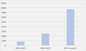
Growth of the number of hits on Google Scholar for the phrase “bandit algorithms”.
Fine, so maybe you decided to care about bandit problems. But what are they exactly? Bandit problems were introduced by William R. Thompson (one of our heroes, whose name we will see popping up again soon) in a paper in 1933 for the so-called Bayesian setting (that we will also talk about later). Thompson was interested in medical trials and the cruelty of running a trial “blindly”, without adapting the treatment allocations on the fly as the drug appears more or less effective.
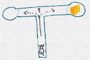
Mice learning in a T-maze
Clinical trials is thus one of the first intended applications. But why would anyone call problems like optimizing drug allocation a “bandit-problem”? The name comes from the 1950s when Frederick Mosteller and Robert Bush decided to study animal learning and ran trials on mice and then on humans. The mice faced the dilemma of choosing to go left or right, after starting in the bottom of a T-shaped maze, not knowing each time at which end they will find food. To study a similar learning setting in humans, a “two-armed bandit” machine was commissioned where humans could choose to pull either the left or the right arm of the machine, each giving a random payoff with the distribution of payoffs for each arm unknown to the human player. The machine was called a “two-armed bandit” in homage to the one-armed bandit, an old-fashioned name for a lever operated slot machine (“bandit” because they steal your money!).

Human facing a two-armed bandit
Now, imagine that you are playing on this two-armed bandit machine and you already pulled each lever 5 times, resulting in the following payoffs:
Left arm: 0, 10, 0, 0, 10
Right arm: 10, 0, 0, 0, 0
The left arm appears to be doing a little better: The average payoff for this arm is 4 (say) dollars per round, while that of the right arm is only 2 dollars per round. Let’s say, you have 20 more trials (pulls) altogether. How would you pull the arms in the remaining trials? Will you keep pulling the left arm, ignoring the right (owing to its initial success), or would you pull the right arm a few more times, thinking that maybe the initial poorer average payoff is due to “bad luck” only? This illustrates the interest in bandit problems: They capture the fundamental dilemma a learner faces when choosing between uncertain options. Should one explore an option that looks inferior or should one exploit one’s knowledge and just go with the currently best looking option? How to maintain the balance between exploration and exploitation is at the heart of bandit problems.
The language of bandits
There are many real-world problems where a learner repeatedly chooses between options with uncertain payoffs with the sole goal of maximizing the total gain over some period of time. However, the world is a messy place. To gain some principled understanding of the learner’s problem, we will often make extra modelling assumptions to restrict how the rewards are generated. To be able to talk about these assumptions, we need a more formal language. In this formal language we are talking about the learner as someone (or something) that interacts with an environment as shown in the figure below.
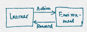
Learner Environment Interaction
On the figure the learner is a represented by a box on the left, the environment is represent by a box on the right. They are interconnected by two arrows connecting the two boxes. These arrows represent the interaction between the learner and the environment. What the figure fails to capture is that the interaction happens in a sequential fashion over a number of discrete rounds. In particular, the specification starts with the following interaction protocol:
For rounds $t=1,2,…,n$:
1. Learner chooses an action $A_t$ from a set $\cA$ of available actions. The chosen action is sent to the environment;
2. The environment generates a response in the form of a real-valued reward $X_t\in \R$, which is sent back to the learner.
The goal of the learner is to maximize the sum of rewards that it receives, $\sum_{t=1}^n X_t$.
A couple of things need to be clarified that are hidden by the above short description: When in step 2 we say that the reward is sent back to the learner, we mean that the learner gets to know this number and can thus use it in the future rounds when it needs to decide which action to take. Thus, in step 1 of round $t$, the learner’s decision is based on the history of interaction up to the end of round $t-1$, i.e., on $H_{t-1} = (A_1,X_1,\dots,A_{t-1},X_{t-1})$.
Our goal, is to equip the learner with a learning algorithm to maximize its reward. Most of the time, the word “algorithm” will not be taken too seriously in the sense that a “learning algorithm” will be viewed as a mapping of possible histories to actions (possibly randomized). Nevertheless, throughout the course we will keep an eye on discussing whether such maps can be efficiently implemented on computers (justifying the name “algorithms”).
The next question to discuss is how to evaluate a learner (to simplify language, we identify learners and learning algorithms)? One idea is to measure learning speed by what is called the regret. The regret of a learner acting in an environment is relative to some action. We will start with a very informal definition (and hope you forgive us). The reason is that there a number of related definitions – all quite similar – and we do not want to be bogged down with the details in this introductory post.
The regret of learner relative to action $a$ =
Total reward gained when $a$ is used for all $n$ rounds –
Total reward gained by the specific learner in $n$ rounds according to its chosen actions.
We often calculate the worst-case regret over the possible actions $a$, though in stochastic environments, we may first take expectations for each action and then calculate the worst-case over the actions (later we should come back to discussing the difference between taking the expectation first and then the maximum, versus taking the maximum first and then the expectation). For a fixed environment, the worst-case regret is just a shift and a sign change of the total reward: Maximizing reward is the same as minimizing regret.
A good learner achieves sublinear worst-case regret: That is, if $R_n$ is the regret after $n$ rounds of interaction of a learner, $R_n = o(n)$. In other words, the average per round regret, $R_n/n$ converges to zero as $n\to\infty$. Of major interest will be to see the rate of growth of regret for various classes of environments, as well as for various algorithms, and in particular, seeing how small the regret can be over some class of environment and what algorithms can achieve such regret lower bounds.
The astute reader may notice that regret compares payoffs of fixed actions to the total payoff of the learner: In particular, in a non-stationary environment, a learner that can change what action it uses over time may achieve negative worst-case regret! In other words, the assumption that the world is stationary (i.e., there are no seasonality or other patterns in the environment, there is no payoff drift, etc.) is built into the above simple concept of regret. The notion of regret can and has been extended to make it more meaningful in non-stationary environments, but as a start, we should be content with the assumption of stationarity. Another point of discussion is whether in designing a learning algorithm we can use the knowledge of the time horizon $n$ or not. In some learning settings assuming this is perfectly fine (say, businesses can have natural business cycles, say, weeks, months, etc.), but sometimes assuming the knowledge of the time horizon is unnatural. In those cases we will be interested in algorithms that work well in lack of the knowledge of the time horizon, in other words, also known as anytime algorithms. As we will see, sometimes the knowledge of time horizon will make a difference when it comes to designing learning algorithms, though usually we find that the difference will be small.
Let’s say we are fine with stationarity. Still, why should one use (worst-case) regret as opposed to simply resorting to comparing learners by the total reward they collected, especially since we said that minimizing the regret is the same as maximizing total reward? Why complicate matters with talking about regret then? First, regret facilitates comparisons across environments by doing a bit of normalization: One can shift rewards by an arbitrary constant amount in some environment and the regret does not change, whereas total reward would be impacted by this change (note that scale is still an issue: multiplying the rewards by a positive constant number, the regret also gets multiplied, so usually we assume some fixed scale, or we need to normalize regret with the scale of rewards). More important however is that regret is well aligned with the intuition that learning should be easy in environments where either (i) all actions pay similar amounts (all learners do well in such environments and all of them will have low regret), and also in environments where (ii) some actions pay significantly more than others (because in such environments it is easy to find the high-paying action or actions, so many learners will have small regret). As a result, the worst-case regret over various classes of environment is a meaningful quantity, as opposed to worst-case total reward which is vacuous. Generally, regret allows one to study learning in worst-case settings. Whether this leads to conservative behavior is another interesting point for further discussion (and is an active topic of research).
With this, let me turn to discussing the typical restrictions on the bandit environments. A particularly simple, yet appealing and rich problem setting is that of stochastic, stationary bandits. In this case the environment is restricted to generate the reward in response to each action from a distribution that is specific to that action, and independently of the previous action choices (of the possibly randomizing learner) and rewards. Sometimes, this is also called “stochastic i.i.d.” bandits since for a given action, any reward for that action is independent of all the other rewards of the same action and they are all generated from identical distributions (that is, there is one distribution per action). Since “stochastic, stationary” and “stochastic i.i.d.” are a bit too long, in the future, we will just refer to this setting as that of “stochastic bandits“. This is the problem setting that we will start discussing next week.
For some applications the assumption that the rewards are generated in a stochastic and stationary way may be too restrictive. In particular, stochastic assumptions can be hard to justify in the real-world: The world, for most of what we know about it, is deterministic, if it is hard to predict and often chaotic looking. Of course, stochasticity has been enormously successful to explain mass phenomenon and patterns in data and for some this may be sufficient reason to keep it as the modeling assumption. But what if the stochastic assumptions fail to hold? What if they are violated for a single round? Or just for one action, at some rounds? Will all our results become suddenly vacuous? Or will the algorithms developed be robust to smaller or larger deviations from the modeling assumptions? One approach, which is admittedly quite extreme, is to drop all the assumptions on how rewards are assigned to arms. More precisely, some minimal assumptions are kept, like that the rewards lie in a bounded interval, or that the reward assignment is done before the interaction begins, or simultaneously with the choice of the learner’s action. In any case, if these are the only assumptions, we get what is called the setting of adversarial bandits. Can we still say meaningful things about the various algorithms? Can learning algorithms achieve nontrivial results? Can their regret be sublinear? It turns out, that, perhaps surprisingly, this is possible. At a second thought though this may not be that surprising: After all, sublinear regret requires only that the learner uses the single best action (best in hindsight) for most of the time, but the learner can still use any other actions for a smaller (and vanishing) fraction of time. What saves learners then is that the identity of the action with the highest total payoff in hindsight cannot change too abruptly and too often as averages cannot be changed too much as long as the summands in the average are bounded.
Course contents
Let’s close with what the course will cover. The course will have three major blocks. In the first block, we will discuss finite-armed bandits, both stochastic and adversarial as these help the best to develop our basic intuition of what makes a learning algorithm good. In the next block we will discuss the beautiful developments in linear bandits, again, both stochastic and adversarial, their connection to contextual bandits, and also various combinatorial settings, which are of major interest in various applications. The reason to spend much time on linearity is because it is the simplest structure that permits one to address large scale problems, and is a very popular and successful modelling assumption. In the last block, we will discuss partial monitoring and learning and acting in Markovian Decision Processes, that is, topics which go beyond bandit problems. With this little excursion outside of bandit land we hope to give a better glimpse for everyone on how exactly bandits fit the bigger picture of online learning under uncertainty.
References and additional reading
The paper by Thompson that was the first to consider bandit problems is the following:
- William R. Thompson. On the likelihood that one unknown probability exceeds another in view of the evidence of two samples. Biometrika, 1933.
Besides Thompson’s seminal paper, there are already a number of books on bandits that may serve as useful additional reading. The most recent (and also most related) is by Sebastien Bubeck and Nicolo Cesa-Bianchi and is freely available online. This is an excellent book and is warmly recommended. The book largely overlaps the topics we will cover, though we are also planning to cover developments that did not fit the page limit of Seb and Nicolo’s book, as well as newer developments.
There are also two books that focus mostly on the Bayesian setting, which we will address only a little. Both are based on relatively old material, but are still useful references for this line of work and are well worth reading.

This is just a test to see whether comments are working.
Oh, let’s see whether MathJax is functional: $\int f(x) dx$.
Greetings from Colorado! I’m bored to death at work so I decided to browse your website on my iphone during lunch
break. I enjoy the knowledge you provide here and
can’t wait to take a look when I get home. I’m surprised at how quick your blog loaded on my
cell phone .. I’m not even using WIFI, just 3G .. Anyways, fantastic site! http://yahoo.co.uk
Great! Who made the wonderful drawings? 🙂
Great that you like them:) The person with the tablet made them.
I will ask my daughter maybe she will accept to contribute to your blog 😉
nit: Is this correct?
“… That is, if $R_n$ is the regret after $n$ rounds of interaction of a learner, $R_n=o(n)$. In other words, the average per round regret, $R_n/n$ converges to zero as n→∞”. $R_n=2n$ is $o(n)$ and $R_n/n$ converges to 2 as $n$ goes to infinity.
$R_n = 2n$ is $O(n)$ (“Big-O”), but not $o(n)$ (“little-o”). This is called Bachmann-Landau notation and there are a variety of other classifications (wiki page explains nicely).
I see, thanks for the explanation!
This series is very useful. Thank you so much for doing this !
Thanks Sharan, we are happy that you found the site useful!
Any thoughts on the O’REILLY book Bandit Algorthms for Website Optimization?
http://shop.oreilly.com/product/0636920027393.do
Hi,
Sorry for the slow reply. Yes, I have checked out this book beforehand and while I cannot say I read it, I glimpsed through it and read some of the explanations that I was curious about. To summarize, I think this is a very fine short, yet informative book. The algorithms are introduced through their actual python codes and the code is explained in details. There are three algorithms discussed and compared in the book: epsilon-greedy, a version of UCB and Exp3. The language is plain and simple, and the book will be most appealing to people who prefer to understand this field by looking at the code of the algorithms instead of starring at mathematical formulae. I found many of the explanation thoughtful and the book seems to be generally careful about delicate matters. Given the constraints on its length, of course, the book could not go into details of why things work and a number of more advanced, yet practically important topics (linear, contextual bandits and beyond). Also some finer distinctions between the algorithms had to be left out too, so people who care about understanding these will need to continue their journey elsewhere. I can recommend the book for everyone with a basic programming background and who are new to bandits. And I really like the direct, simple approach taken. Good job John Myles White (the author of the book)!
Cheers,
Csaba
Apparently the equations produced by MathJax don’t show up properly on Instapaper or Pocket. Anyone know a fix for this or some alternative that works better?
Would it work to read a pdf? You can print the whole contents to pdf (Chrome does this very nicely) and then read it offline. Unfortunately, you need to choose a “paper size”, but maybe this is better than nothing.
Hi! Thank you for this high-quality work. Here is some feedback:
# Applications and origin
> or would you pull the right arm a few more times, thinking that maybe the initial poorer average payoff is due to “bad luck” only?
You could illustrate this notion of “bad luck” by plotting an example of probability distribution for each arm and where the 5 first pulls fall.
# The language of bandits
> For a fixed environment, the worst-case regret is just a shift and a sign change of the total reward: Maximizing reward is the same as minimizing regret.
I’ve struggled with this, probably because I cannot understand the regret intuitively. What’s the point of looking at what happens when we keep taking the same action?
You could make this sentence clearer by being more explicit: “For a deterministic environment, the total reward gained when a is used for all n rounds is constant, so the worst-case regret is just…”.
> A good learner achieves sublinear worst-case regret: That is, if Rn is the regret after n rounds of interaction of a learner, Rn=o(n).
I don’t understand this. Is it a definition of a good learner?
> The astute reader may notice that regret compares payoffs of fixed actions
The term “fixed” is ambiguous here as you use it above as “deterministic” (“For a fixed environment, the worst-case regret is just a shift and a sign change of the total reward”).
> In particular, in a non-stationary environment
Sounds risky to assume the reader is familiar with this notion of stationarity.
Thanks!
Re regret and comparing with a fixed action: I assume you are fine with the goal that the learner should maximize the total expected reward. Now, if the learner knew the environment, what would they do? Notice that in this case in every round the learner could just pull the action that gives the highest mean reward. The regret just asks: Compared this optimal behavior, which assume a bit too much (knowledge of which arm gives the maximum mean payoff), how much does the learner loses in terms of the mean reward? A kind of half-empty (rather than half-full) mentality. The reason the regret is preferred is because we want to compare how a single learner behaves across different environments. If two environments differ only by that all rewards are just shifted, if we used the total expected reward collected, the performance of a learner looks better in the environment whose rewards were upshifted by some positive number. For example, environment B has the same rewards as environment A plus 10. Now the learner looks better in environment B. But this is not because of the skillfulness of the learner, but because the environment just has higher rewards. To prevent this kind of misleading information, it is better to compare learners based on how they performance relative to the optimal strategy that uses the full information about the environment. I hope this explanation cleans up this concern. Also note that the environments do not need to be deterministic! If we care about the expected total reward, even in a stochastic environment, the optimal strategy is to keep pulling the action with the highest mean reward.
Re sublinear regret and the definition of good learners: Yes, this was meant to be a minimum requirement for what a good learner should aim for.
Re next mention of fixed action: I hope my explanation to the first concern clears this up, too.
Stationary, non-stationary: Yes, we were ahead of ourselves here, though this particular paragraph is luckily not essential for understanding the rest. In the book, we have a separate chapter dealing with nonstationary environments, which could also help. I am not sure whether you are looking for an explanation here, but just in case, by stationary we simply meant that the laws governing the response of the environment (how rewards are generated in response to the learner pulling arms) do not change over time. Then, nonstationarity is just when this does not hold.