Lower bounds for linear bandits turn out to be more nuanced than the finite-armed case. The big difference is that for linear bandits the shape of the action-set plays a role in the form of the regret, not just the distribution of the noise. This should not come as a big surprise because the stochastic finite-armed bandit problem can be modeled as a linear bandit with actions being the standard basis vectors, $\cA = \set{e_1,\ldots,e_K}$. In this case the actions are orthogonal, which means that samples from one action do not give information about the rewards for other actions. Other action sets such as the sphere ($\cA = S^d = \{x \in \R^d : \norm{x}_2 = 1\}$) do not share this property. For example, if $d = 2$ and $\cA = S^d$ and an algorithm chooses actions $e_1 = (1,0)$ and $e_2 = (0,1)$ many times, then it can deduce the reward it would obtain from choosing any other action.

We will prove a variety of lower bounds under different assumptions. The first three have a worst-case flavor showing what is (not) achievable in general, or under a sparsity constraint, or if the realizable assumption is not satisfied. All of these are proven using the same information-theoretic tools that we have seen for previous results, combined with careful choices of action sets and environment classes. The difficulty is always in guessing what is the worst case, which is followed by simply turning the cranks on the usual machinery.

Besides the worst-case results we also give an optimal asymptotic lower bound for finite action sets that generalizes the asymptotic lower bound for finite-armed stochastic bandits give in a previous post. The proof of this result is somewhat more technical, but follows the same general flavor as the previous asymptotic lower bounds.

We use a simple model with Gaussian noise. For action $A_t \in \cA \subseteq \R^d$ the reward is $X_t = \shortinner{A_t, \theta} + \eta_t$ where $\eta_t\sim \mathcal N(0,1)$ is the standard Gaussian noise term and $\theta \in \Theta \subset \R^d$. The regret of a strategy is:
\begin{align*}
R_n(\cA, \theta) = \max_{x \in \cA} \E\left[\sum_{t=1}^n \shortinner{x^* – A_t, \theta}\right]\,,
\end{align*}
where $x^* = \argmax_x \shortinner{x, \theta}$ is the optimal action. Note that the arguments to the regret function differ from those used in some previous posts. In general we include the quantities of interest, which in this case (with a fixed strategy and noise model) are the action set and the unknown parameter. As for finite-armed bandits we define the sub-optimality gap of arm $x \in \cA$ by $\Delta_x = \max_{y \in \cA} \shortinner{y – x, \theta}$ and $\Delta_{\min} = \inf \set{\Delta_x : x \in \cA \text{ and } \Delta_x > 0}$. Note that the latter quantity can be zero if $\cA$ is infinitely large, but is non-zero if there are finitely many arms and the problem is non-trivial (there exists a sub-optimal arm). If $A$ is a matrix, then $\lambda_{\min}(A)$ is its smallest eigenvalue. We also recall the notation used for finite-armed bandits by defining $T_x(t) = \sum_{s=1}^t \one{A_s = x}$.

Worst case bounds

Our worst case bound relies on a specific action set and shows that the $\tilde O(d \sqrt{n})$ upper bound for linear version of UCB cannot be improved in general except (most likely) for the logarithmic factors.

Theorem Let the action set be $\mathcal A = \set{-1, 1}^d$. Then for any strategy there exists a $\theta \in \Theta = \set{-\sqrt{1/n}, \sqrt{1/n}}^d$ such that
\begin{align*}
R_n(\cA, \theta) \geq \frac{\exp(-2)}{4} \cdot d \sqrt{n}\,.
\end{align*}

Proof
For $\theta \in \Theta$ we denote $\mathbb{P}_\theta$ to be the measure on outcomes $A_1, X_1,\ldots,A_n,X_n$ induced by the interaction of the strategy and the bandit determined by $\theta$. By the relative entropy identity we have for $\theta, \theta’ \in \Theta$ that
\begin{align}
\KL(\mathbb{P}_\theta, \mathbb{P}_{\theta’}) = \frac{1}{2} \sum_{t=1}^n \E\left[\shortinner{A_t, \theta – \theta’}^2\right]\,.
\label{eq:linear-kl}
\end{align}
For $1 \leq i \leq d$ and $\theta \in \Theta$ define
\begin{align*}
p_{\theta,i} = \mathbb{P}_\theta\left(\sum_{t=1}^n \one{\sign(A_{t,i}) \neq \sign(\theta_i)} \geq n/2\right)\,.
\end{align*}
Now let $1 \leq i \leq d$ and $\theta \in \Theta$ be fixed and let $\theta’ = \theta$ except for $\theta’_i = -\theta_i$. Then by the high probability version of Pinsker’s inequality and (\ref{eq:linear-kl}) we have
\begin{align}
\label{eq:sphere-kl}
p_{\theta,i} + p_{\theta’,i}
&\geq \frac{1}{2} \exp\left(-\frac{1}{2}\sum_{t=1}^n \shortinner{A_t, \theta – \theta’}^2\right)
= \frac{1}{2} \exp\left(-2\right)\,.
\end{align}
Therefore using the notation $\sum_{\theta_{-i}}$ as an abbreviation for $\sum_{\theta_1,\ldots,\theta_{i-1},\theta_{i+1},\ldots,\theta_d \in \set{\pm \sqrt{1/n}}^{d-1}}$,
\begin{align*}
\sum_{\theta \in \Theta} 2^{-d} \sum_{i=1}^d p_{\theta,i}
&= \sum_{i=1}^d \sum_{\theta_{-i}} 2^{-d} \sum_{\theta_i \in \set{\pm \sqrt{1/n}}} p_{\theta,i} \\
&\geq \sum_{i=1}^d \sum_{\theta_{-i}} 2^{-d} \cdot \frac{1}{2}\exp\left(-2\right) \\
&= \frac{d}{4} \exp\left(-2\right)\,.
\end{align*}
Therefore there exists a $\theta \in \Theta$ such that
\begin{align*}
\sum_{i=1}^d p_{\theta,i} \geq \frac{d}{4} \exp\left(-2\right)\,.
\end{align*}
Let $x^* = \argmax_{x \in \cA} \shortinner{x^*, \theta}$. Then by the definition of $p_{\theta,i}$, the regret for this choice of $\theta$ is at least
\begin{align*}
R_n(\cA, \theta)
&= \sum_{t=1}^n \E_\theta\left[\shortinner{x^* – A_t, \theta}\right] \\
&= 2\sqrt{\frac{1}{n}} \sum_{i=1}^d \sum_{t=1}^n \mathbb{P}_\theta\left(\sign(A_{t,i}) \neq \sign(\theta_i)\right) \\
&\geq \sqrt{n} \sum_{i=1}^d \mathbb{P}_\theta\left(\sum_{t=1}^n \one{\sign(A_{t,i}) \neq \sign(\theta_i)} \geq n/2 \right) \\
&= \sqrt{n} \sum_{i=1}^d p_{\theta,i}
\geq \frac{\exp(-2)}{4} \cdot d \sqrt{n}\,.
\end{align*}
QED

Sparse case

We now tackle the sparse case where the underlying parameter $\theta$ is assumed to have $\norm{\theta}_0 = \sum_{i=1}^d \one{\theta_i > 0} \leq p$ for some $p$ that is usually much smaller than $d$. An extreme case is when $p= 1$, which essentially reduces to the finite-armed bandit problem where we observe the regret is at least $\Omega(\sqrt{dn})$ in the worst case. For this reason we cannot expect too much from sparsity. It turns out that the best one can hope for (in the worst case) is $\Omega(\sqrt{p d n})$, so again the lower bound is nearly matching the upper bound for an existing algorithm.

Theorem
Let $2 \leq p\leq d$ be even and define the set of actions $\cA$ by
\begin{align*}
\mathcal A = \set{ x \in \set{0, 1}^d : \sum_{i=1}^d \one{x_i > 0} = \frac{p}{2}}.
\end{align*}
Then for any strategy there exists a $\theta$ with $\norm{\theta}_0 \leq p$ such that
\begin{align*}
R_n \geq \frac{\sqrt{2d p n}}{16} \exp(-1)\,.
\end{align*}

The assumption that $p$ is even is non-restrictive, since in case it is not even the following proof goes through for $p – 1$ and the regret only changes by a very small constant factor. The proof relies on a slightly different construction than the previous result, and is fractionally more complicated because of it.

Proof
Let $\epsilon = \sqrt{2d/(p n)}$ and $\theta$ be given by
\begin{align*}
\theta_i = \begin{cases}
\epsilon\,, & \text{if } i \leq p / 2\,; \\
0\,, & \text{otherwise}\,.
\end{cases}
\end{align*}
Given $S \subseteq \{p/2+1,\ldots,d\}$ with $|S| = p/2$ define $\theta’$ by
\begin{align*}
\theta’_i = \begin{cases}
\epsilon\,, & \text{if } i \leq p / 2\,; \\
2\epsilon\,, & \text{if } i \in S \,; \\
0\,, & \text{otherwise}\,.
\end{cases}
\end{align*}
Let $\mathbb{P}_\theta$ and $\mathbb{P}_{\theta’}$ be the measures on the sequence of observations when a fixed strategy interacts with the bandits induced by $\theta$ and $\theta’$ respectively. Then the usual computation shows that
\begin{align*}
\KL(\mathbb{P}_\theta, \mathbb{P}_{\theta’}) = 2\epsilon^2 \E\left[\sum_{t=1}^n \sum_{i \in S} \one{A_{ti} \neq 0}\right]\,.
\end{align*}
By the pigeonhole principle we can choose an $S \subseteq \{p/2+1,\ldots,d\}$ with $|S| = p/2$ in such a way that
\begin{align*}
\E\left[\sum_{t=1}^n \sum_{i \in S} \one{A_{ti} \neq 0}\right] \leq \frac{n p}{d}\,.
\end{align*}
Therefore using this $S$ and with the high probability pinsker we have for any event $A$ that
\begin{align*}
\mathbb{P}_\theta(A) + \mathbb{P}_{\theta’}(A^c) \geq \frac{1}{2} \exp\left(-\KL(\mathbb{P}_\theta, \mathbb{P}_{\theta’})\right)
\geq \frac{1}{2} \exp\left(-\frac{np\epsilon^2}{2d}\right)
\geq \frac{1}{2} \exp\left(-1\right)
\end{align*}
Choosing $A = \set{\sum_{t=1}^n \sum_{i \in S} \one{A_{ti} > 0} \geq np/4}$ leads to
\begin{align*}
R_n(\mathcal A, \theta) &\geq \frac{n\epsilon p}{4} \mathbb{P}_{\theta}(A) &
R_n(\mathcal A, \theta’) &\geq \frac{n\epsilon p}{4} \mathbb{P}_{\theta’}(A^c)\,.
\end{align*}
Therefore
\begin{align*}
\max\set{R_n(\cA, \theta),\, R_n(\cA, \theta’)}
\geq \frac{n\epsilon p}{8} \left(\mathbb{P}_{\theta}(A) + \mathbb{P}_{\theta’}(A^c)\right)
\geq \frac{\sqrt{2ndp}}{16} \exp(-1)\,.
\end{align*}
QED

Unrealizable case

An important generalization of the linear model is the unrealizable case where the mean rewards are not assumed to follow a linear model exactly. Suppose that $\cA \subset \R^d$ and the mean reward is $\E[X_t|A_t = x] = \mu_x$ does not necessarily satisfy a linear model. It would be very pleasant to have an algorithm such that if $\mu_x = \shortinner{x, \theta}$ for all $x$, then
\begin{align*}
R_n(\cA, \mu) = \tilde O(d \sqrt{n})\,,
\end{align*}
while if there exists an $x \in \cA$ such that $\mu_x \neq \shortinner{x, \theta}$, then $R_n(\cA, \mu) = \tilde O(\sqrt{nK})$ recovers the UCB bound. That is, an algorithm that enjoys the bound of OFUL if the the linear model is correct, but recovers the regret of UCB otherwise. Of course one could hope for something even stronger, for example that
\begin{align}
R_n(\cA, \mu) = \tilde O\left(\min\set{\sqrt{Kn},\, d\sqrt{n} + n\epsilon}\right)\,, \label{eq:hope}
\end{align}
where $\epsilon = \min_{\theta \in \R^d} \max_{x \in \cA} |\mu_x – \shortinner{x, \theta}|$ is called the approximation error of the class of linear models. Unfortunately it turns out that results of this kind are not achievable. To show this we will prove a generic bound for the classical finite-armed bandit problem, and then show how this implies a lower bound on the ability to be adaptive to a linear model if possible and have acceptable regret if not.

Theorem
Let $\cA = \set{e_1,\ldots,e_K}$ be the standard basis vectors. Now define sets $\Theta, \Theta’ \subset \R^{K}$ by
\begin{align*}
\Theta &= \set{\theta \in [0,1]^K : \theta_i = 0 \text{ for } i > 1} \\
\Theta’ &= \set{\theta \in [0,1]^K}\,.
\end{align*}
If $2(K-1) \leq V \leq \sqrt{n(K-1)\exp(-2)/8}$ and $\sup_{\theta \in \Theta} R_n(\cA, \theta) \leq V$, then
\begin{align*}
\sup_{\theta’ \in \Theta’} R_n(\cA, \theta’) \geq \frac{n(K-1)}{8V} \exp(-2)\,.
\end{align*}

Proof
Let $\theta \in \Theta$ be given by $\theta_1 = \Delta = (K-1)/V \leq 1/2$. Therefore
\begin{align*}
\sum_{i=2}^K \E[T_i(n)] \leq \frac{V}{\Delta}
\end{align*}
and so by the pigeonhole principle there exists an $i > 1$ such that
\begin{align*}
\E[T_i(n)] \leq \frac{V}{(K-1)\Delta} = \frac{1}{\Delta^2}\,.
\end{align*}
Then define $\theta’ \in \Theta’$ by
\begin{align*}
\theta’_j = \begin{cases}
\Delta & \text{if } j = 1 \\
2\Delta & \text{if } j = i \\
0 & \text{otherwise}\,.
\end{cases}
\end{align*}
Then by the usual argument for any event $A$ we have
\begin{align*}
\mathbb{P}_\theta(A) + \mathbb{P}_{\theta’}(A^c)
\geq \frac{1}{2} \exp\left(\KL(\mathbb{P}_\theta, \mathbb{P}_{\theta’})\right)
= \frac{1}{2} \exp\left(-2 \Delta^2 \E[T_i(n)]\right)
\geq \frac{1}{2} \exp\left(-2\right)\,.
\end{align*}
Therefore
\begin{align*}
R_n(\mathcal A, \theta) + R_n(\mathcal A, \theta’)
\geq \frac{n\Delta}{4} \exp(-2) = \frac{n(K-1)}{4V} \exp(-2)
\end{align*}
Therefore by the assumption that $R_n(\mathcal A, \theta) \leq V \leq \sqrt{n(K-1) \exp(-2)/8}$ we have
\begin{align*}
R_n(\mathcal A, \theta’) \geq \frac{n(K-1)}{8V} \exp(-2)\,.
\end{align*}
Therefore $R_n(\cA, \theta) R_n(\cA, \theta’) \geq \frac{n(K-1)}{8} \exp(-2)$ as required.
QED

As promised we now relate this to the unrealizable linear bandits. Suppose that $d = 1$ (an absurd case) and that there are $K$ arms $\cA = \set{x_1, x_2,\ldots, x_{K}}$ where $x_1 = (1)$ and $x_i = (0)$ for $i > 1$. Clearly if the reward is really linear and $\theta > 0$, then the first arm is optimal, while otherwise any of the other arms have the same expected reward (of just $0$). Now simply add $K-1$ coordinates to each action so that the error in the 1-dimensional linear model can be modeled in a higher dimension and we have exactly the model used in the previous theorem. So $\cA = \set{e_1,e_2,\ldots,e_K}$. Then the theorem shows that (\ref{eq:hope}) is a pipe dream. If $R_n(\cA, \theta) = \tilde O(\sqrt{n})$ for all $\theta \in \Theta’$ (the realizable case), then there exists a $\theta’ \in \Theta’$ such that $R_n(\cA, \theta’) = \tilde \Omega(K \sqrt{n})$. To our knowledge it is still an open question of what is possible on this front. Our conjecture is that there is an algorithm for which
\begin{align*}
R_n(\cA, \theta) = \tilde O\left(\min\set{d\sqrt{n} + \epsilon n,\, \frac{K}{d}\sqrt{n}}\right)\,.
\end{align*}
In fact, it is not hard to design an algorithm that tries to achieve this bound by assuming the problem is realizable, but using some additional time to explore the remaining arms up to some accuracy to confirm the hypothesis. We hope to write a post on this in the future, but leave the claim as a conjecture for now.

Asymptotic lower bounds

Like in the finite-armed case, the asymptotic result is proven only for consistent strategies. Recall that a strategy is consistent in some class if the regret is sub-polynomial for any bandit in that class.

Theorem Let $\cA \subset \R^d$ be a finite set that spans $\R^d$ and suppose a strategy satisfies
\begin{align*}
\text{for all } \theta \in \R^d \text{ and } p > 0 \qquad R_n(\cA, \theta) = o(n^p)\,.
\end{align*}
Let $\theta \in \R^d$ be any parameter such that there is a unique optimal action and let $\bar G_n = \E_\theta \left[\sum_{t=1}^n A_t A_t^\top\right]$ be the expected Gram matrix when the strategy interacts with the bandit determined by $\theta$. Then $\liminf_{n\to\infty} \lambda_{\min}(\bar G_n) / \log(n) > 0$ (which implies that $\bar G_n$ is eventually non-singular). Furthermore, for any $x \in \cA$ it holds that:
\begin{align*}
\limsup_{n\to\infty} \log(n) \norm{x}_{\bar G_n^{-1}}^2 \leq \frac{\Delta_x^2}{2}\,.
\end{align*}

The reader should recognize $\norm{x}_{\bar G_n^{-1}}^2$ as the key term in the width of the confidence interval for the least squares estimator. This is quite intuitive. The theorem is saying that any consistent algorithm must prove statistically that all sub-optimal arms are indeed sub-optimal. Before the proof of this result we give a corollary that characterizes the asymptotic regret that must be endured by any consistent strategy.

Corollary
Let $\cA \subset \R^d$ be a finite set that spans $\R^d$ and $\theta \in \R^d$ be such that there is a unique optimal action. Then for any consistent strategy
\begin{align*}
\liminf_{n\to\infty} \frac{R_n(\cA, \theta)}{\log(n)} \geq c(\cA, \theta)\,,
\end{align*}
where $c(\cA, \theta)$ is defined as
\begin{align*}
&c(\cA, \theta) = \inf_{\alpha \in [0,\infty)^{\cA}} \sum_{x \in \cA} \alpha(x) \Delta_x \\
&\quad\text{ subject to } \norm{x}_{H_\alpha^{-1}}^2 \leq \frac{\Delta_x^2}{2} \text{ for all } x \in \cA \text{ with } \Delta_x > 0\,,
\end{align*}
where $H = \sum_{x \in \cA} \alpha(x) x x^\top$.

Proof of Theorem
The proof of the first part is simply omitted (see the reference below for details). It follows along similar lines to what follows, essentially that if $G_n$ is not “sufficiently large” in every direction, then some alternative parameter is not sufficiently identifiable. Let $\theta’ \in \R^d$ be an alternative parameter and let $\mathbb{P}$ and $\mathbb{P}’$ be the measures on the sequence of outcomes $A_1,Y_1,\ldots,A_n,Y_n$ induced by the interaction between the strategy and the bandit determined by $\theta$ and $\theta’$ respectively. Then for any event $E$ we have
\begin{align}
\Prob{E} + \mathbb{P}'(E^c)
&\geq \frac{1}{2} \exp\left(-\KL(\mathbb{P}, \mathbb{P}’)\right) \nonumber \\
&= \frac{1}{2} \exp\left(-\frac{1}{2} \E\left[\sum_{t=1}^n \inner{A_t, \theta – \theta’}^2\right]\right)
= \frac{1}{2} \exp\left(-\frac{1}{2} \norm{\theta – \theta’}_{\bar G_n}^2\right)\,. \label{eq:linear-asy-kl}
\end{align}
A simple re-arrangement shows that
\begin{align*}
\frac{1}{2} \norm{\theta – \theta’}_{\bar G_n}^2 \geq \log\left(\frac{1}{2 \Prob{E} + 2 \mathbb{P}'(E^c)}\right)
\end{align*}
Now we follow the usual plan of choosing $\theta’$ to be close to $\theta$, but so that the optimal action in the bandit determined by $\theta’$ is not $x^*$. Let $\epsilon \in (0, \Delta_{\min})$ and $H$ be a positive definite matrix to be chosen later such that $\norm{x – x^*}_H^2 > 0$. Then define
\begin{align*}
\theta’ = \theta + \frac{\Delta_x + \epsilon}{\norm{x – x^*}^2_H} H(x – x^*)\,,
\end{align*}
which is chosen so that
\begin{align*}
\shortinner{x – x^*, \theta’} = \shortinner{x – x^*, \theta} + \Delta_x + \epsilon = \epsilon\,.
\end{align*}
This means that $x^*$ is not the optimal action for bandit $\theta’$, and in fact is $\epsilon$-suboptimal. We abbreviate $R_n = R_n(\cA, \theta)$ and $R_n’ = R_n(\cA, \theta’)$. Then
\begin{align*}
R_n
&= \E_\theta\left[\sum_{x \in \cA} T_x(n) \Delta_x\right]
\geq \frac{n\Delta_{\min}}{2} \Prob{T_{x^*}(n) < n/2} \geq \frac{n\epsilon}{2} \Prob{T_{x^*}(n) < n/2}\,. \end{align*} Similarly, $x^*$ is at least $\epsilon$-suboptimal in bandit $\theta'$ so that \begin{align*} R_n' \geq \frac{n\epsilon}{2} \mathbb{P}'\left(T_{x^*}(n) \geq n/2\right)\,. \end{align*} Therefore \begin{align} \Prob{T_{x^*}(n) < n/2} + \mathbb{P}'\left(T_{x^*}(n) \geq n/2\right) \leq \frac{2}{n\epsilon} \left(R_n + R_n'\right)\,. \label{eq:regret-sum} \end{align} Note that this holds for practically any choice of $H$ as long as $\norm{x - x^*}_H > 0$. The logical next step is to select that $H$ (which determines $\theta’$) in such a way that (\ref{eq:linear-asy-kl}) is as large as possible. The main difficulty is that this depends on $n$, so instead we aim to choose an $H$ so the quantity is large enough infinitely often. We starting by just re-arranging things:
\begin{align*}
\frac{1}{2} \norm{\theta – \theta’}_{\bar G_n}^2
= \frac{(\Delta_x + \epsilon)^2}{2} \cdot \frac{\norm{x – x^*}_{H \bar G_n H}^2}{\norm{x-x^*}_H^4}
= \frac{(\Delta_x + \epsilon)^2}{2 \norm{x – x^*}_{\bar G_n^{-1}}^2} \rho_n(H)\,,
\end{align*}
where we introduced
\begin{align*}
\rho_n(H) = \frac{\norm{x – x^*}_{\bar G_n^{-1}}^2 \norm{x – x^*}_{H \bar G_n H}^2}{\norm{x – x^*}_H^4}\,.
\end{align*}
Therefore by choosing $E$ to be the event that $T_{x^*}(n) < n/2$ and using (\ref{eq:regret-sum}) and (\ref{eq:linear-asy-kl}) we have \begin{align*} \frac{(\Delta_x + \epsilon)^2}{2\norm{x - x^*}_{\bar G_n^{-1}}^2} \rho_n(H) \geq \log\left(\frac{n \epsilon}{4R_n + 4R_n'}\right)\,, \end{align*} which after re-arrangement leads to \begin{align*} \frac{(\Delta_x + \epsilon)^2}{2\log(n)\norm{x - x^*}_{\bar G_n^{-1}}^2} \rho_n(H) \geq 1 - \frac{\log((4R_n + 4R_n')/\epsilon)}{\log(n)}\,. \end{align*} The definition of consistency means that $R_n$ and $R_n'$ are both sub-polynomial, which implies that the second term in the previous expression tends to zero for large $n$ and so by sending $\epsilon$ to zero we see that \begin{align} \label{eq:lin-lower-liminf} \liminf_{n\to\infty} \frac{\rho_n(H)}{\log(n) \norm{x - x^*}_{\bar G_n^{-1}}^2} \geq \frac{2}{\Delta_x^2}\,. \end{align} We complete the result using proof by contradiction. Suppose that \begin{align} \limsup_{n\to\infty} \log(n) \norm{x - x^*}_{\bar G_n^{-1}}^2 > \frac{\Delta_x^2}{2}\,. \label{eq:linear-lower-ass}
\end{align}
Then there exists an $\epsilon > 0$ and infinite set $S \subseteq \N$ such that
\begin{align*}
\log(n) \norm{x – x^*}_{\bar G_n^{-1}}^2 \geq \frac{(\Delta_x + \epsilon)^2}{2} \quad \text{ for all } n \in S\,.
\end{align*}
Therefore by (\ref{eq:lin-lower-liminf}),
\begin{align*}
\liminf_{n \in S} \rho_n(H) > 1\,.
\end{align*}
We now choose $H$ to be a cluster point of the sequence $\{\bar G_n^{-1} / \norm{\bar G_n^{-1}}\}_{n \in S}$ where $\norm{\bar G_n^{-1}}$ is the spectral norm of the matrix $\bar G_n^{-1}$. Such a point must exist, since matrices in this sequence have unit spectral norm by definition, and the set of matrices with bounded spectral norm is compact. We let $S’ \subseteq S$ be a subset so that $\bar G_n^{-1} / \norm{\bar G_n^{-1}}$ converges to $H$ on $n \in S’$. We now check that $\norm{x – x^*}_H > 0$.
\begin{align*}
\norm{x – x^*}_H^2 = \lim_{n \in S} \frac{\norm{x – x^*}^2_{\bar G_n^{-1}}}{\norm{\bar G_n^{-1}}}
> 0\,,
\end{align*}
where the last inequality follows from the assumption in (\ref{eq:linear-lower-ass}) and the first part of the theorem. Therefore
\begin{align*}
1 < \liminf_{n \in S} \rho_n(H) \leq \liminf_{n \in S'} \frac{\norm{x - x^*}^2_{\bar G_n^{-1}} \norm{x - x^*}^2_{H \bar G_n^{-1}H}}{\norm{x - x^*}_H^4} = 1\,, \end{align*} which is a contradiction, and so we conclude that (\ref{eq:linear-lower-ass}) does not hold and so \begin{align*} \limsup_{n\to\infty} \log(n) \norm{x - x^*}_{\bar G_n^{-1}}^2 \leq \frac{\Delta_x^2}{2}\,. \end{align*} QED

We leave the proof of the corollary as an exercise for the reader. Essentially though, any consistent algorithm must choose its actions so that in expectation
\begin{align*}
\norm{x – x^*}^2_{\bar G_n^{-1}} \leq (1 + o(1)) \frac{\Delta_x^2}{2 \log(n)}\,.
\end{align*}
Now since $x^*$ will be chosen linearly often it is easily shown for sub-optimal $x$ that $\lim_{n\to\infty} \norm{x – x^*}_{\bar G_n^{-1}} / \norm{x}_{\bar G_n^{-1}} \to 1$. This leads to the required constraint on the actions of the algorithm, and the optimization problem in the corollary is derived by minimizing the regret subject to this constraint.

Clouds looming for optimism

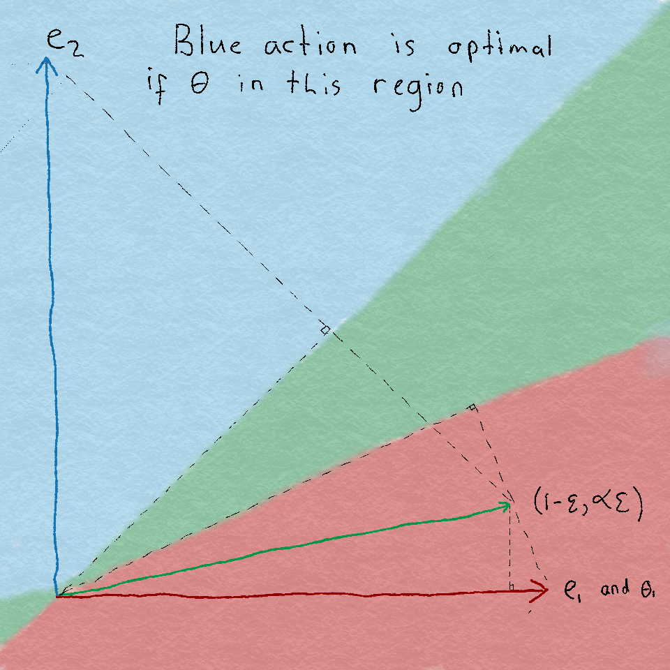
The theorem and its corollary have disturbing implications for strategies based on the principle of optimism in the face of uncertainty, which is that they can never be asymptotically optimal! The reason is that these strategies do not choose actions for which they have collected enough statistics to prove they are sub-optimal, but in the linear setting it can still be worthwhile playing these actions in case they are very informative about other actions for which the statistics are not yet so clear. A problematic example appears in the simplest case where any information sharing between the arms occurs at all. Namely, when the dimension is $d = 2$ and there are $K = 3$ arms.

Specifically, let $\cA = \set{x_1, x_2, x_3}$ where $x_1 = e_1$ and $x_2 = e_2$ and $x_3 = (1-\epsilon, \gamma \epsilon)$ where $\gamma \geq 1$ and $\epsilon > 0$ is small. Let $\theta = (1, 0)$ so that the optimal action is $x^* = x_1$ and $\Delta_{x_2} = 1$ and $\Delta_{x_3} = \epsilon$. Clearly if $\epsilon$ is very small, then $x_1$ and $x_3$ point in nearly the same direction and so choosing only these arms does not yield which of $x_1$ or $x_3$ is optimal. On the other hand, $x_2$ and $x_1 – x_3$ point in very different directions and so choosing $x_2$ allows a learning agent to quickly identify that $x_1$ is in fact optimal.

We now show how the theorem and corollary demonstrate this. First we calculate what is the optimal solution to the optimization problem. Recall we are trying to minimize
\begin{align*}
\sum_{x \in \cA} \alpha(x) \Delta_x \qquad \text{subject to } \norm{x}^2_{H(\alpha)^{-1}} \leq \frac{\Delta_x^2}{2} \text{for all } x \in \cA\,,
\end{align*}
where $H = \sum_{x \in \cA} \alpha(x) x x^\top$. Clearly we should choose $\alpha(x_1)$ arbitrarily large, then a computation shows that
\begin{align*}
\lim_{\alpha(x_1) \to \infty} H(\alpha)^{-1} =
\left[\begin{array}{cc}
0 & 0 \\
0 & \frac{1}{\alpha(x_3)\epsilon^2 \gamma^2 + \alpha(x_2)}
\end{array}\right]\,.
\end{align*}
Then for the constraints mean that
\begin{align*}
&\frac{1}{\alpha(x_3)\epsilon^2 \gamma^2 + \alpha(x_2)} = \lim_{\alpha(x_1) \to \infty} \norm{x_2}^2_{H(\alpha)^{-1}} \leq \frac{1}{2} \\
&\frac{\gamma^2 \epsilon^2}{\alpha(x_3) \epsilon^2 \gamma^2 + \alpha(x_2)} = \lim_{\alpha(x_1) \to \infty} \norm{x_3}^2_{H(\alpha)^{-1}} \leq \frac{\epsilon^2}{2}\,.
\end{align*}
Provided that $\gamma \geq 1$ this reduces simply to the constraint that
\begin{align*}
\alpha(x_3) \epsilon^2 + \alpha(x_2) \geq 2\gamma^2\,.
\end{align*}
Since we are minimizing $\alpha(x_2) + \epsilon \alpha(x_3)$ we can easily see that $\alpha(x_2) = 2\gamma^2$ and $\alpha(x_3) = 0$ provided that $2\gamma^2 \leq 2/\epsilon$. Therefore if $\epsilon$ is chosen sufficiently small relative to $\gamma$, then the optimal rate of the regret is $c(\cA, \theta) = 2\gamma^2$ and so there exists a strategy such that
\begin{align*}
\limsup_{n\to\infty} \frac{R_n(\cA, \theta)}{\log(n)} = 2\gamma^2\,.
\end{align*}
Now we argue that for $\gamma$ sufficiently large and $\epsilon$ arbitrarily small that the regret for any consistent optimistic algorithm is at least
\begin{align*}
\limsup_{n\to\infty} \frac{R_n(\cA, \theta)}{\log(n)} = \Omega(1/\epsilon)\,,
\end{align*}
which can be arbitrarily worse than the optimal rate! So why is this so? Recall that optimistic algorithms choose
\begin{align*}
A_t = \argmax_{x \in \cA} \max_{\tilde \theta \in \cC_t} \inner{x, \tilde \theta}\,,
\end{align*}
where $\cC_t \subset \R^d$ is a confidence set that we assume contains the true $\theta$ with high probability. So far this does not greatly restrict the class of algorithms that we might call optimistic. We now assume that there exists a constant $c > 0$ such that
\begin{align*}
\cC_t \subseteq \set{\tilde \theta : \norm{\hat \theta_t – \tilde \theta}_{G_t} \leq c \sqrt{\log(n)}}\,.
\end{align*}
So now we ask how often can we expect the optimistic algorithm to choose action $x_2 = e_2$ in the example described above? Since we have assumed $\theta \in \cC_t$ with high probability we have that
\begin{align*}
\max_{\tilde \theta \in \cC_t} \shortinner{x_1, \tilde \theta} \geq 1\,.
\end{align*}
On the other hand, if $T_{x_2}(t-1) > 4c^2 \log(n)$, then
\begin{align*}
\max_{\tilde \theta \in \cC_t} \shortinner{x_2, \tilde \theta}
&= \max_{\tilde \theta \in \cC_t} \shortinner{x_2, \tilde \theta – \theta} \\
&\leq 2 c \sqrt{\norm{x_2}_{G_t^{-1}} \log(n)} \\
&\leq 2 c \sqrt{\frac{\log(n)}{T_{x_2}(t-1)}} \\
&< 1\,, \end{align*} which means that $x_2$ will not be chosen more than $1 + 4c^2 \log(n)$ times. So if $\gamma = \Omega(c^2)$, then the optimistic algorithm will not choose $x_2$ sufficiently often and a simple computation shows it must choose $x_3$ at least $\Omega(\log(n)/\epsilon^2)$ times and suffers regret of $\Omega(\log(n)/\epsilon)$. The key take-away from this is that optimistic algorithms do not choose actions that are statistically sub-optimal, but for linear bandits it can be optimal to choose these actions more often to gain information about other actions.

Notes

Note 1: The worst-case bound demonstrates the near-optimality of the OFUL algorithm for a specific action-set. It is an open question to characterize the optimal regret for a wide range of action-sets. We will return to these issues soon when we discuss adversarial linear bandits.

Note 2: There is an algorithm that achieves the asymptotic lower bound (see references below), but so far there is no algorithm that is simultaneously asymptotically optimal and (near) minimax optimal.

Note 3: The assumption that $x^*$ was unique in the asymptotic results can be relaxed at the price of a little more work, and simple (natural) modifications to the theorem statements.

References

Worst-case lower bounds for stochastic bandits have appeared in a variety of places, all with roughly the same bound, but for different action sets. Our very simple proof is new, but takes inspiration mostly from the paper by Shamir.

• Dani, Hayes and Kakade. Stochastic Linear Optimization under Bandit Feedback, 2008.
• Rusmevichientong and Tsitsiklis. Linearly Parameterized Bandits, 2010.
• Shamir. On the Complexity of Bandit Linear Optimization, 2014.

The asymptotic lower bound (along with a strategy for which the upper bound matches) is by the authors.

• Lattimore and Szepesvari. The End of Optimism? An Asymptotic Analysis of Finite-Armed Linear Bandits, 2016.

The example used to show optimistic approaches cannot achieve the optimal rate has been used before in the pure exploration setting where the goal is to simply find the best action, without the constraint that the regret should be small.

• Soare, Lazaric, Munos. Best-Arm Identification in Linear Bandits, 2015.

We should also mention that examples have been constructed before demonstrating the need for carefully balancing the trade-off between information and regret. For many examples, and a candidate design principle for addressing these issues see

• Russo & Van Roy. Learning to Optimize via Information-Directed Sampling, 2014.

The results for the unrealizable case are inspired by the work of one of the authors on the pareto regret frontier for bandits, which characterizes what trade-offs are available when it is desirable to have a regret that is unusually small relative to some specific arms.

• Lattimore. The Pareto Regret Frontier for Bandits, 2015.